Introduction
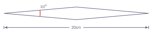
 In this exercise the flow past a symmetrical diamond wedge airfoil will be calculated using the commercial software STAR-CCM+. The geometry and grid generation, as well as the solution of the Navier-Stokes equations that describe the flow, is carried out within the same software. The wedge chord is 20 cm and the leading and trailing edge angle is 10\(^\circ\). Below is a drawing of the wedge
OBS! Read chapter 4 in the course book before starting this exercise.
When you have done the assignment, you should write a short report and hand in for assessment of this course element (instructions at the bottom of this page).
Working remotely
If you decide that you prefer to work remotely instead of on campus, remote access to Chalmers computers is possible. Instructions on how to remotely access Chalmers Linux computers can be found in the following links (depending on your computer’s operative system):
Preparatory calculations
Before the computer session starts, some hand calculations need to be performed in order to, for instance, be able to specify correct values for the boundary conditions on the CFD software. Also, a comparison between the analytically obtained forces and moments on the wedge and the ones obtained numerically will be performed. Calculate the force (x and y components) that the fluid exerts on the wedge assuming that the air behaves as an ideal gas with \(\gamma\) = 1.4 and the following free-stream conditions; \(p_\infty\) = 101325 Pa, \(T_\infty\) = 300 K, an angle of attack of 3\(^\circ\) and Mach number equal to 2.5. Viscous effects might be neglected. Also compute the axial location where the moment is zero.
Do the preparatory calculations before getting started with STAR-CCM+!
Assignment guide
In this section a step by step guide is given so that you can simulate the flow over the wedge, going from geometry generation and meshing, all the way to simulating and post-processing.
Note! in the following, RC denotes mouse right click
Getting started
In order to launch STAR-CCM+, open a new terminal window and type star-ccm+ to start the software. To start a new simulation, click File −> New. In that menu you can select Serial under Process Options, and in the License section click on Power on Demand and copy the Power-on-Demand Key that can be found in the file POD.txt published on Canvas.
Geometry generation
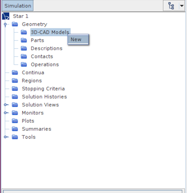
Next step is to open the built in CAD module to generate and prepare the geometry. In order to do so:
Geometry −> RC 3D-CAD Models −> New
Once the 3D CAD modeler is opened, rename the domain by right clicking 3D-CAD Model 1 and Rename, in this case Fluid domain seems like a suitable name. Now we need to create a sketch where we will draw the wedge geometry as well as the computational domain boundaries. To do that:
RC XY −> Create Sketch
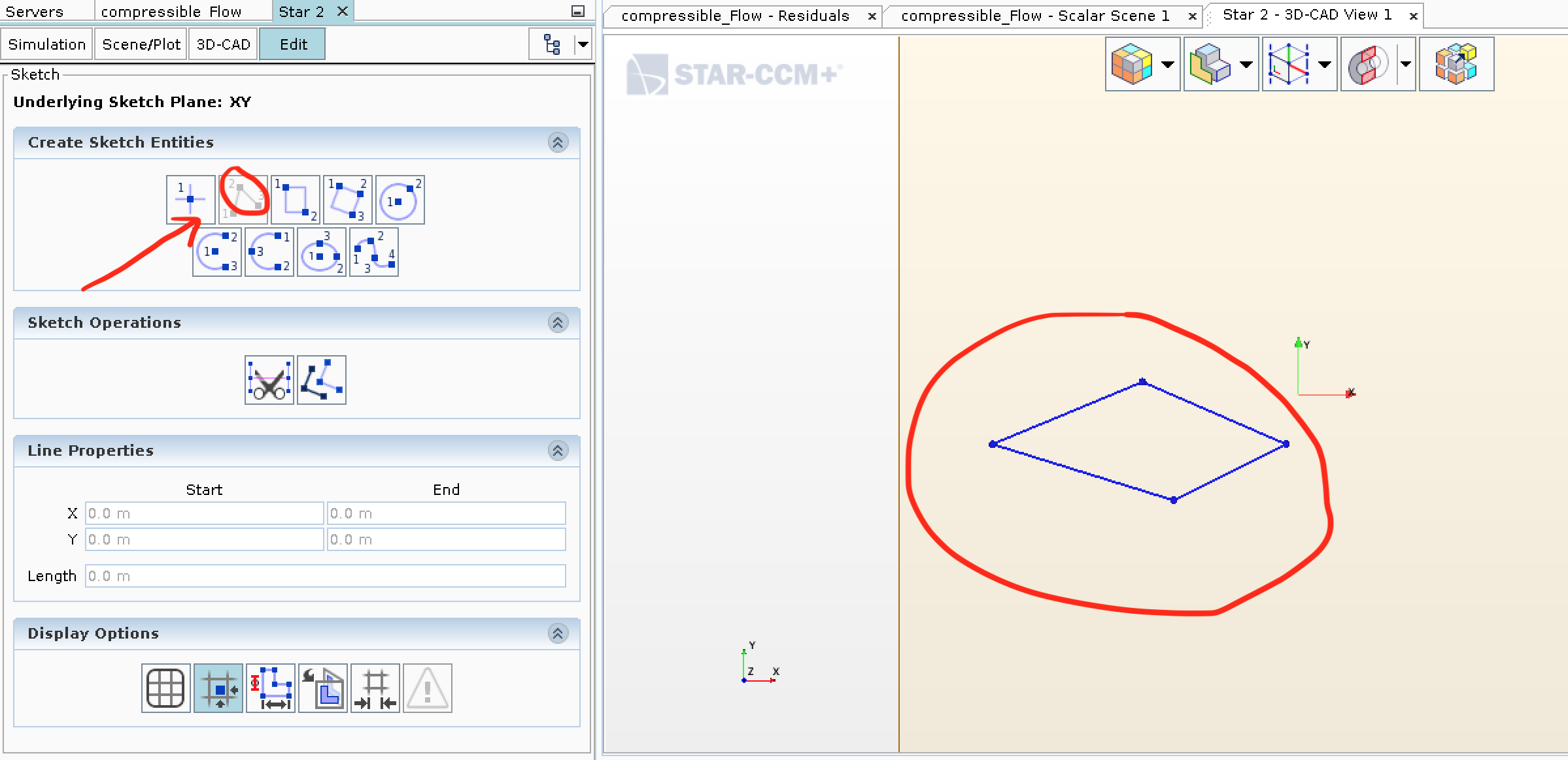
Click on the Create Line option (see figure below) and draw a four-sided closed polygon by clicking on the sketching area (the actual location of the points/lines is not important as it will be changed later) as can be seen in the figure below,
Once we have created the four sided closed polygon, we will adjust the coordinates to make sure they represent the wedge airfoil we want to simulate. In order to modify the points, click on each of the four lines and modify the values of Start and End under Line Properties in the left menu so that the final coordinates are as follows,
	left point:   x = -0.1 m, y =  0.0 m
	top point:    x =  0.0 m, y =  0.0087489 m
	right point:  x =  0.1 m, y =  0.0 m
	bottom point: x =  0.0 m, y = -0.0087489 m
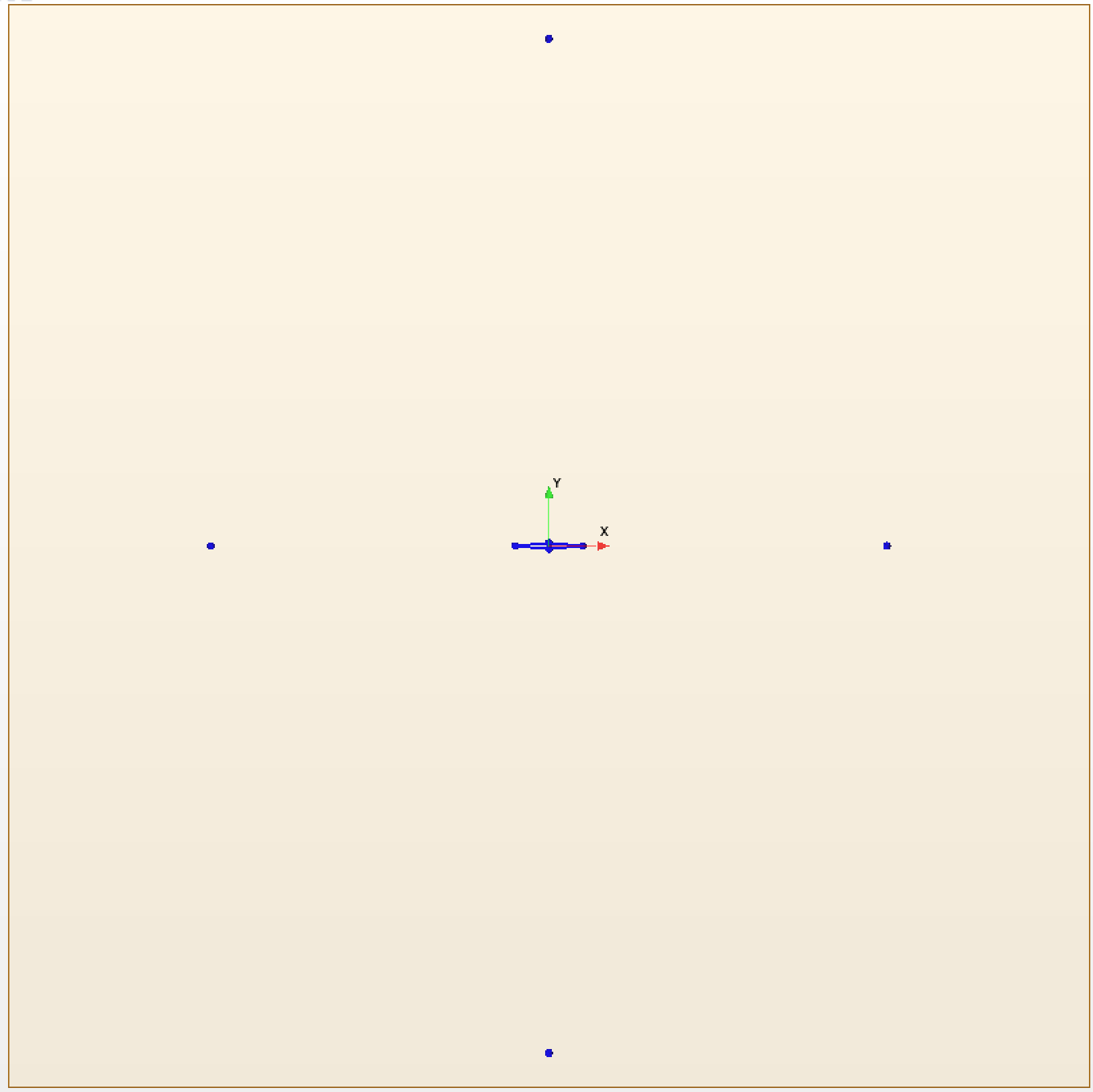
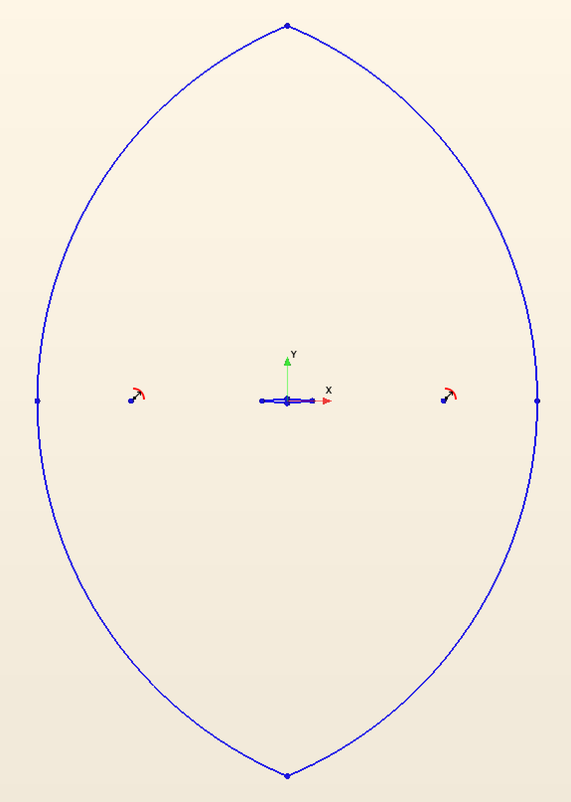
Now that the wedge has been drawn, it is time to create two outer arcs that will define our computational domain boundaries. In order to create a point, click on Create Point in the left menu under Create Sketch Entries and place it somewhere random in the sketch domain. Then, similarly as we did for the wedge lines, click on the recently created point to modify its \(x\) and \(y\) coordinates. Now, Create four points with the following coordinates,
	point 1: x = -1.0 m, y =  0.0 m
	point 2: x =  0.0 m, y =  1.5 m
	point 3: x =  1.0 m, y =  0.0 m
	point 4: x =  0.0 m, y = -1.5 m
The sketch should now look like the one in the figure below.
Last step is to create two arcs joined at the top and the bottom points recently created. To do so, click on Create Three-Point Circular Arc and then click on the end points of the arc (i.e. the top and bottom points) and then in either the right or left point to finish the arc creation. When the two arcs are created, the sketch should look like the figure bellow.
Now that we are done sketching lets go ahead and click on OK. The next step is to extrude the sketch we have just drawn, as STAR-CCM+ requires us to use a 3D geometry.
RC Sketch 1 −> Extrude
Since the depth of the extrusion is of no importance in a 2D simulation, accept the default settings. Now let's rename the surfaces of interest (when the simulation is actually run in 2D these will no longer be surfaces but boundary lines) so that they can be identified when setting up the boundary conditions. Do this by right clicking on the corresponding surface (the surface will turn purple, make sure you have selected a surface and not an edge) and clicking on Rename under Face. The figure below shows how the surfaces should be renamed.
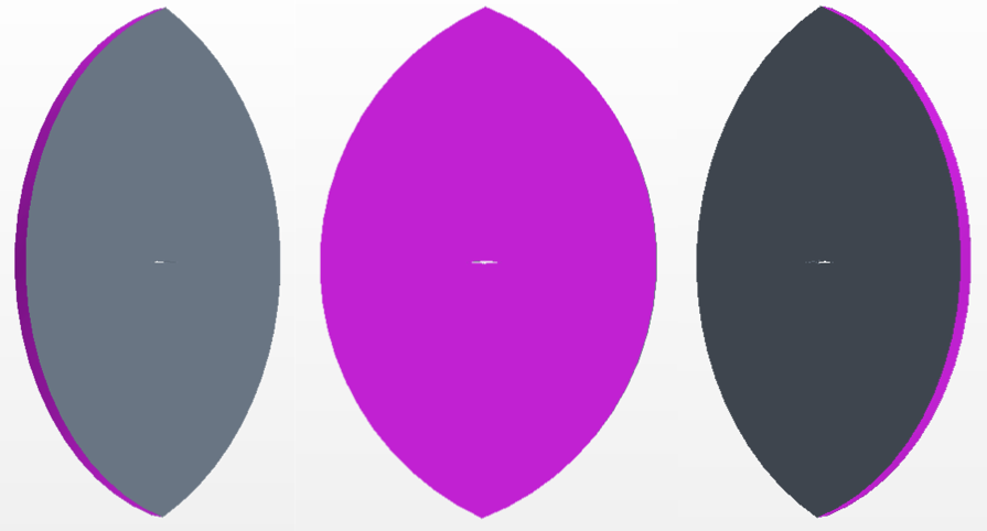
(2dsurf2 surface opposite parallel to 2dsurf1)
Check that the surface naming is correct: Body Groups −> Body 1 −> Named Faces, click on any of the named surfaces and it will be highlighted in the CAD model.
Now the geometry is defined and we can close the CAD module. Press Close 3D-CAD in the lower part of the left hand side model tree.
Finally, the generated geometry should be added to the Fluid domain
Geometry −> 3D-CAD Models −> RC Fluid domain −> New Geometry Part
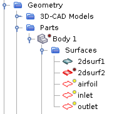
In the popup window, we can accept the default settings and press OK. It can be seen now, that in the left-hand-side model tree, the Geometry -> Parts folder contains the geometry that has been created in the 3D CAD module Body 1 with the renamed faces Body 1 -> Surfaces.
Previously all surfaces were renamed except for the wedge-airfoil itself. The reason for this is that the airfoil is made out of multiple surfaces. Instead of selecting all of them to rename it, the following can be done:
Geometry −> Parts −> Body 1 −> Surfaces −> RC Default −> Rename
Set the default surface name to airfoil. Since all surfaces except the airfoil have
already been named, the surfaces grouped under the Default tag are the airfoil surfaces.
Preparing for the meshing
In the CAD module, the 3D geometry has been created but we want to do a 2D simulation. Therefore, we need to do the following:
Geometry −> RC Operations −> New −> Mesh −> Badge for 2D Meshing
In the pop-up menu that appears, select the small square to the left of Body 1
and click OK.
Notice that under Operations, Badge for 2D Meshing has been added. Right click on it and then click Execute. By doing this STAR-CCM+ has figured out on which plane to generate the surface mesh (2D mesh). If everything worked correctly, a * should be seen on one of the surfaces 2dsurf1 or 2dsurf2 (note that the * can appear in either of the two surfaces) as shown in the figure below.
So far everything has been done under Geometry. To transfer that information to other places of the software (for instance, the Regions folder) so that it can be used by the mesher and the CFD solver, proceed as:
Geometry −> Parts −> RC Body 1 −> Assign Parts to Regions
and configure the Assign Parts to Regions so that it looks like the one in the figure,
click Apply and Close.
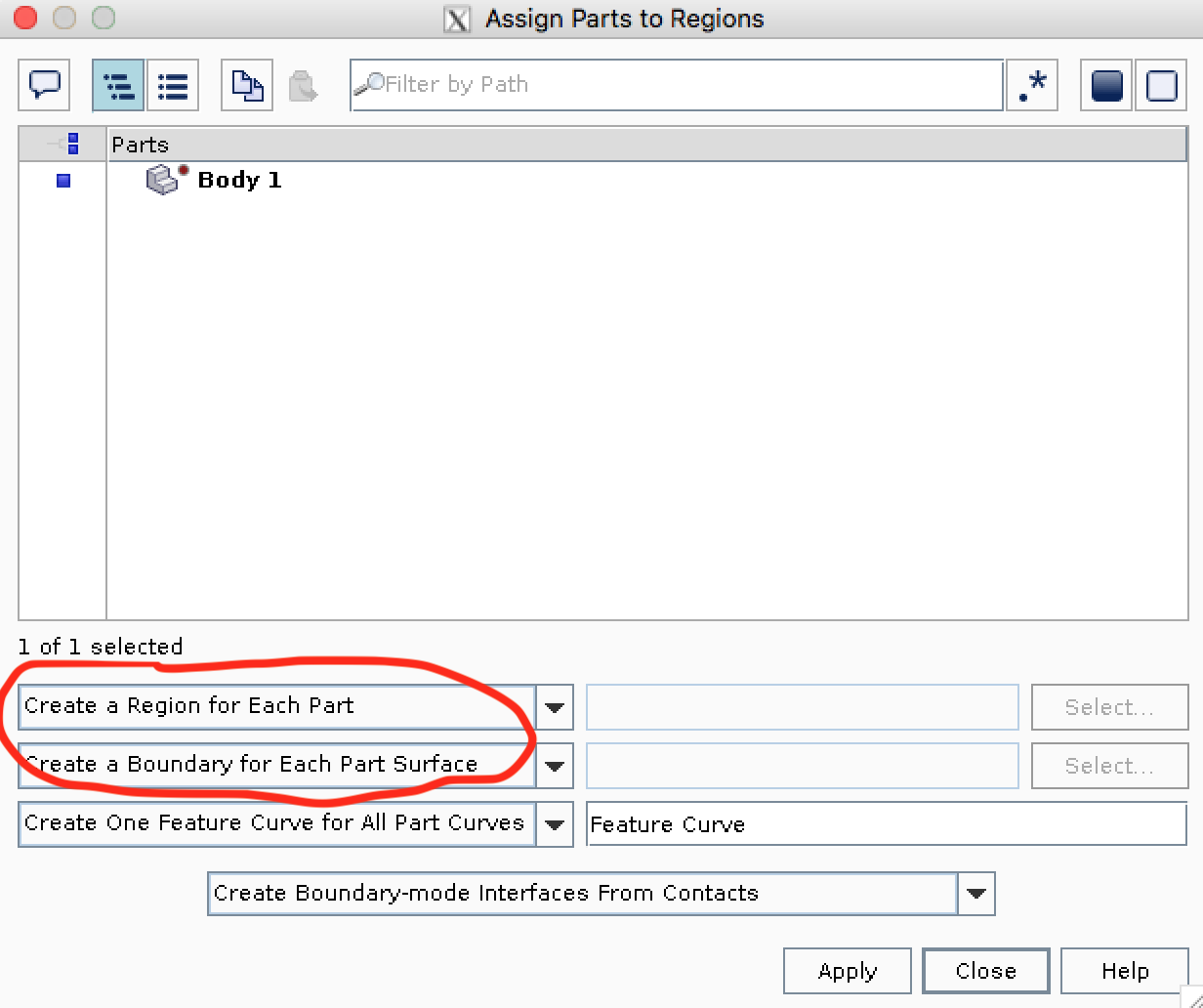
After this, it can be seen that under Regions a lot of new information has appeared, such as all the information about the renamed surfaces.
Meshing
Now that all the necessary information has been provided, let's start to create the computational mesh:
Geometry −> RC Operations −> New −> Mesh −> Automated Mesh (2D)
In the pop window, select Body 1 in the Parts menu and the Polygonal Mesher, click OK. By doing this, STAR-CCM+ knows what type of elements that should be used for the meshing (polygonal).
Under Operations the newly created Automated Mesh (2D) has appeared, unfold it and change the following settings under Default controls (these are some recommendations that are will result in a mesh with good enough quality - feel free to experiment with them):
Base Size −> 0.1 m

Minimum Surface Size −> Perc. of Base −> 100.0

Surface Growth Rate −> 1.05 (OBS! change from Default to User Specified first)
This sets up the basic settings of the mesh, but refinement close to the walls of the airfoil is desired. For that we will create a Custom Control.
Geometry −> Operations −> Automated Mesh (2D) −> RC Custom Controls −> New −> Surface Control
Double click on the new entry under Custom Controls. The parts that need to be modified by this custom control are selected, in this case arfoil. This is done by clicking on the ”three dots” next to Part Surfaces in the pop up menu.
The next set of settings is therefore only applied to the airfoil. By default, the settings are going to be the same as the ones defined in Default Controls. The main different between the airfoil surface and the rest of the domain is the required resolution in order to capture all the flow gradient that will occur there, leading to smaller cell sizes. Change the following settings under the recently created Custom Control −> Surface Control −> Controls:
Target Surface Size −> Custom

Surface Growth Rate −> Custom
and now under Custom Control −> Surface Control −> Values:
Target Surface Size −> Perc. of Base −> 0.5

Surface Growth Rate −> 1.025 (OBS! change from Default to User Specified first)
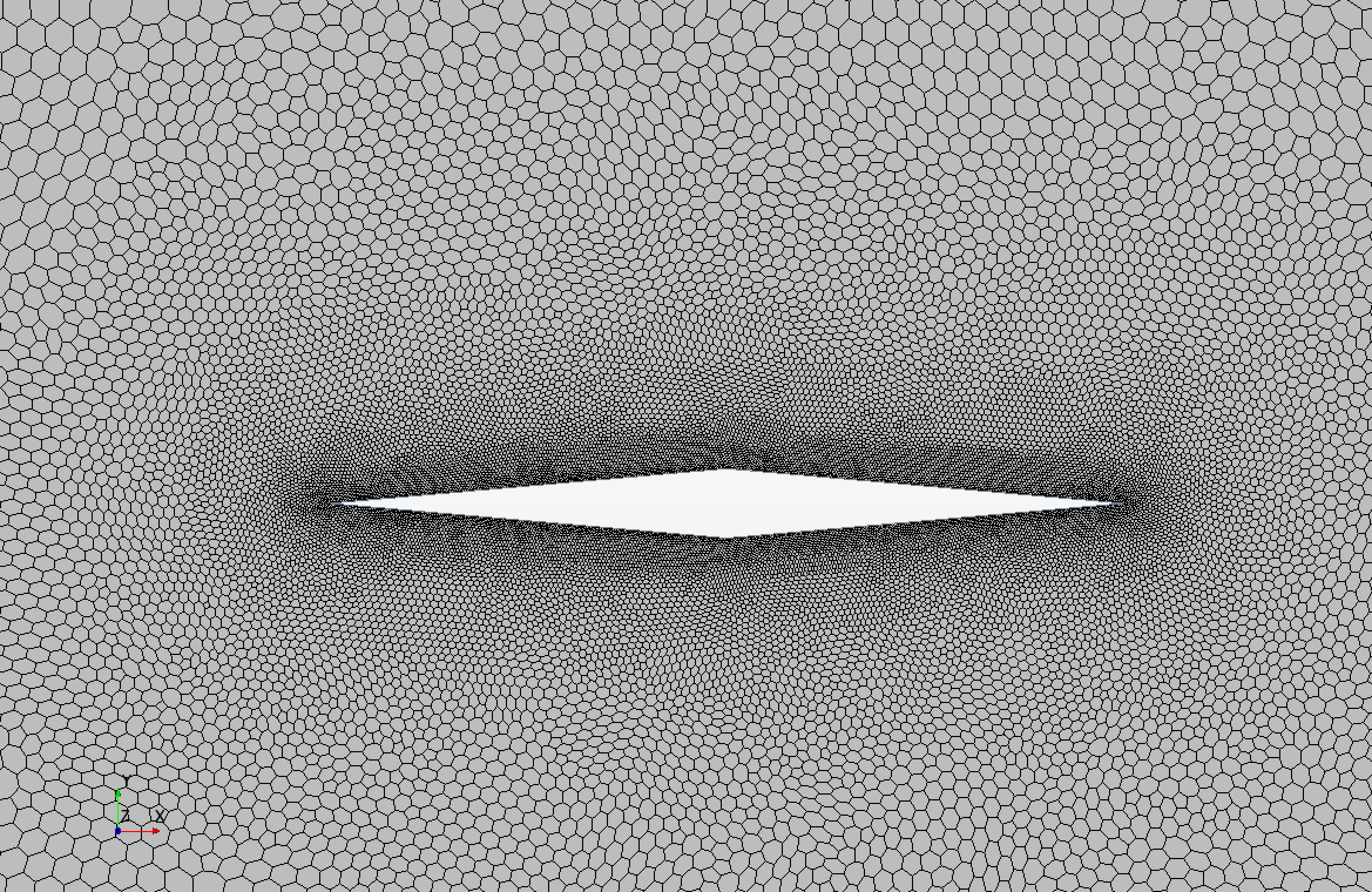
Finally generate and display the mesh by clicking as shown in the figure:
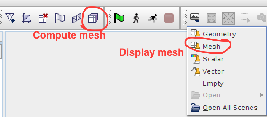
A close up of the mesh around the wedge is shown bellow
Solver settings
First, rename Continua −> Physics 1 to Fluid.
Now it's time to setup the solver environment
Continua −> RC Fluid −> Select Models
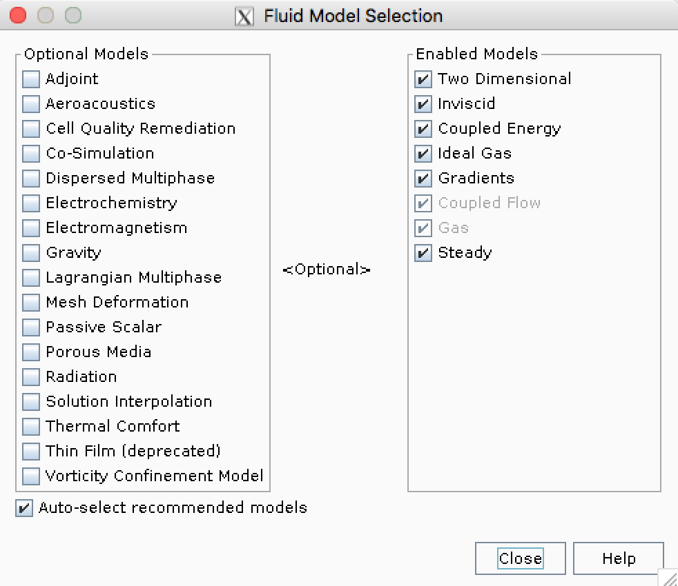
In the pop up menu select the solver settings as follows:
Two dimensional (This might be already selected by default)

Steady

Gas

Coupled Flow

Ideal Gas

Inviscid
After all this has been selected it should look like in the figure below (only the right part should have the same items).
Finally the reference pressure should be set to zero in order to be consistent with the specified \(p_\infty\) and the calculated \(p_o\).
Continua −> Fluid −> Reference Values −> Reference Pressure −> Value = 0.0 Pa
Boundary conditions
First, set the type of boundary conditions that are going to be used in Regions −> Body 1 −> Boundaries as follows:
inlet −> Type −> Stagnation Inlet

outlet −> Type −> Pressure Outlet
The default type is wall, so there is no need to modify airfoil. The boundary conditions of the simulation are going to be set up according to the values you obtained by hand calculation.
Regions −> Body 1 −> Boundaries
and set the following:
inlet
	Physics Conditions −> Flow Direction specification −> Angles
	Physics Values −> Flow Angles −> [angle of attack, 0., 0.]
	Physics Values −> Supersonic Static Pressure −> p_inf
	Physics Values −> Total Pressure −> p_o
	Physics Values -> Total Temperature −> T_o
outlet
	Physics Values −> Pressure −> p_inf
	Physics Values −> Static Temperature −> T_inf
\(p_o\) and \(T_o\) should be computed using the given free-stream conditions.
Initial conditions
Under Continua −> Fluid −> Initial Conditions, specify initial flow conditions as follows:
Static Temperature −> T_inf
Static Pressure −> p_inf
Velocity −> V_inf
\(V_\infty\) should be computed from the given Mach number, angle of attack and \(T_\infty\).
Stopping criteria and monitoring simulation
Now that the simulation is set up, we need to tell STAR-CCM+ when to stop computing. This can be done in different ways. Here, we will set several criteria. The first one being the maximum number of iterations we want to allow STAR-CCM+ to perform. Of course, this does not mean that the solution is convereged when STAR-CCM+ has performed those iterations, but it is an initial guess, more iterations might be needed. The maximum number of iterations is set as follows:
Stopping Criteria −> Maximum Steps −> 1000
Another way to monitor the convergence of the simulation is to check the value of the residuals of each of the equations that are being solved. In this case we are solving four equations, namely, continuity, X-momentum, Y-momentum and energy. A criterion for one of these equations can be set as
RC Stopping Criteria −> New Monitor Criterion...
In the pop-up menu select Continuity and click OK, this will allow us to set a criterion for the continuity equation residual. Under the Stopping Criteria, Continuity Criterion will appear and we can now set it up as follows:
Continuity Criterion −> Logical Rule −> And
Continuity Criterion −> Minimum Limit −> 1.0E-5
In the same way, set convergence criteria for the remaining three equations that are being solved (i.e. energy, X-momentum, and Y-momentum).
Verify that the maximum steps criterion is set as follows:
Stopping Criteria −> Maximum Steps −> Logical Rule −> Or
this means that our stopping criteria will be a mix of all the specified criteria. With this settings STAR-CCM+ will stop iterating if one of the following two things occur, either it reaches the maximum number of steps (the logical rule is OR) or it checks that the residuals for all the four equations is below \(10^{−5}\) (the logical
rule is AND).
Another way of checking whether the simulation has converged or not, is to monitor values that we are interested in. In this case such values could be the forces that the fluid exerts on the wedge-airfoil. A force monitor is set up as follows:
RC Reports −> New Report −> Flow/Energy −> Force
A new report called Force 1 has been created, right click on it and rename it to Force X. Click on the report and under Parts, select airfoil. Now let's bring our attention to the following two settings in the report:
Direction −> [1.0, 0.0, 0.0]
Force Option −> Pressure + Shear
With the direction setting we can set the direction in which the force will be measured, since for this particular report we are interested in the \(x\) direction of the force, the default setting is correct. Under Force Option we have Pressure + Shear by default, in this case, since we are running an inviscid simulation, the Shear part of the force will be zero as there in no viscosity. Therefore setting Force Option to Pressure + Shear or to Pressure will give identical results.
Similarly create a report for the force in Y direction. In order to be able to see how these values change during the iteration, we would like to plot them. To do so, right click on one of the reports and Create Monitor and Plot from Report. If the solution is converged, since we are running steady state, the values of the force monitor should be stable. Do the same for the other force report.
The plots of the monitored variables are placed under Plots, to visualize them (in case they did not become visible automatically) just double click on them.
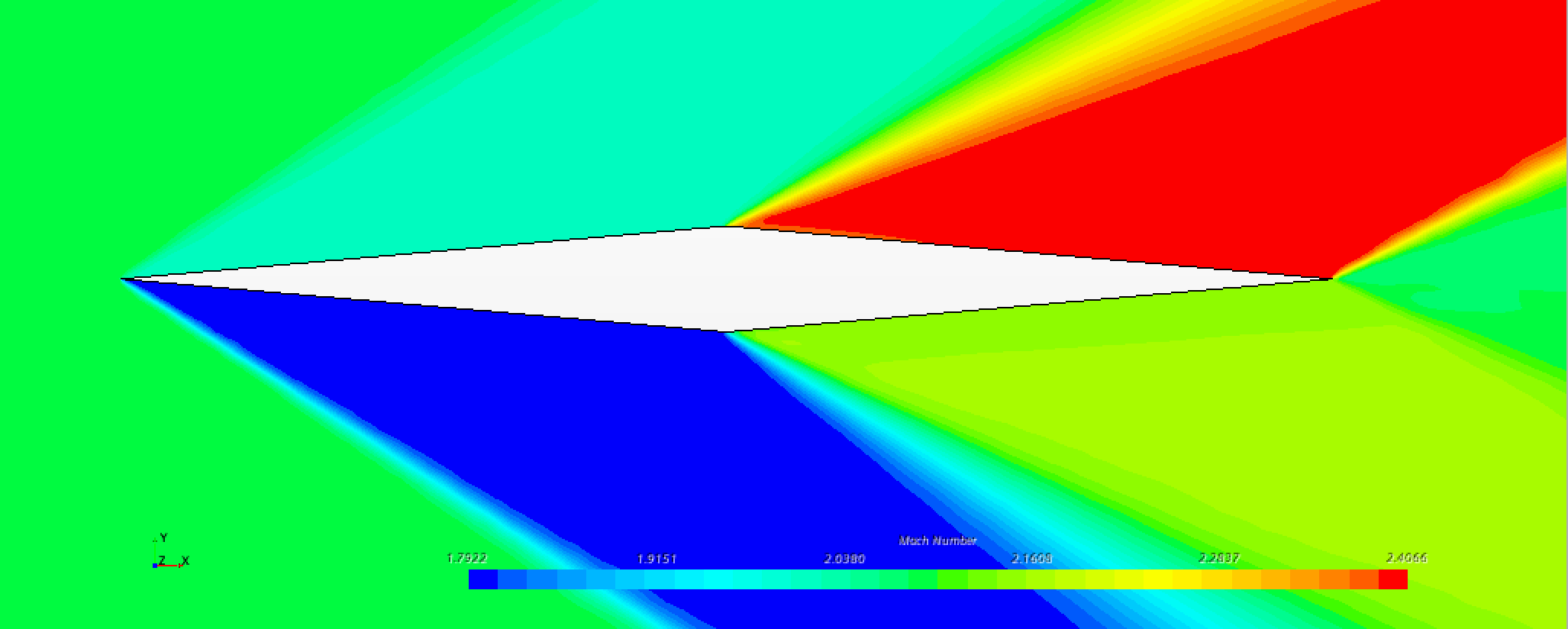
Apart from monitoring variables through plots, contours of variables can be displayed as the simulation is running so that the entire flow field can be visualized. In order to do so, a Scene needs to be created as follows (for instance, the contour of the Mach number):
RC Scenes −> New Scene −> Scalar
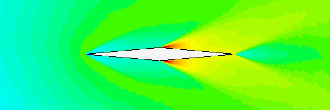
after this, the geometry will pop up in a scalar scene. Right click on the color bar that reads Select Function and select Mach Number. Rename the newly created scene to something meaningful like Mach number. When the simulation begins to run, this contour plot will be automatically refreshed as shown in the figures bolow.
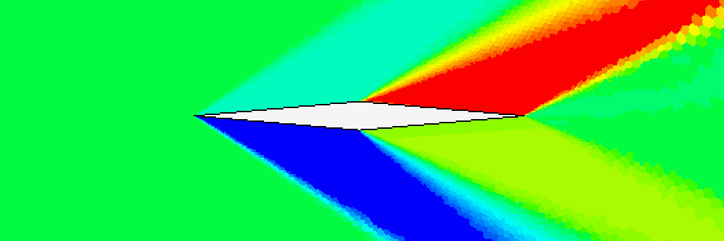
When making a scalar scene the default Contour Style is set to Automatic. This means that the contour is colored by cell value, but it is preferred to have a continuous and smooth contour plot. In order to get smooth contour plots, do as follows:
Scenes −> Mach number −> Scalar 1
In the menu that appears below the left-hand-side model tree, set the Contour Style option to Smooth Filled. The difference between the two contour styles can be seen in the figure below.

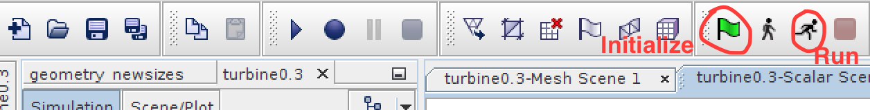
Initializing and running the simulation
Initialize the solution and then on start the simulation by clicking the buttons shown in the figure below.
While the simulation is running you can change what to visualize using the tabs on top of the main visualization window:

Assignment Report
When yoy are done with the simulation, you should write a brief report and hand in in Canvas. The report should include the following:
- Plot Mach number and static pressure, and zoom in on the wedge, comment what you see.
- Report and compare the forces calculated by hand and by STAR-CCM+. How accurate is the CFD simulation?
- Calculate the position where the moment is zero from the forces you calculated by hand. Compare this with STAR-CCM+. In order to compute the moment on STAR-CCM+, create a report in the same way you did for the forces in X and Y direction but instead of
Force, selectMoment. Then in the newly createdMoment 1report you can specify along which axis the moment needs to be computed. You can right click on theMoment 1report and thenRun Reportevery time you change the axis or its origin so that you do not have to simulate everything from scratch. The result will be shown in theOutputwindow. - Make a plot of total pressure and zoom in on the wedge. Comment on what you see!
- When showing the hand calculations, it is enough with taking a picture of the paper or scanning it, no need to type everything down.