 Inviscid compressible flow in 2 space dimensions (\(x\) and \(y\) coordinates) and time is assumed. A geometry according to the picture below is defined and the problem consists of computing numerically the initially unsteady 2D flow developing around a symmetric airfoil (impulsive start), including the expected pressure waves and/or shocks. After some time, the solution obtained should converge towards a steady-state flow.
Additionally, the drag coefficient dependence on Mach-number for the symmetric airfoil is compared to a supercritical airfoil. For drag calculations an additional complication is added: viscosity.
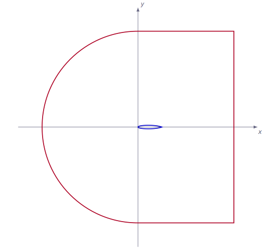
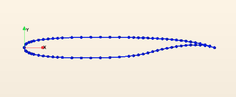
Figure 1 gives a suggested layout for the computational domain. The wing profile is located in the center of the domain (blue lines) and the surrounding mesh extends from -10m to 10m in the \(x\) direction and from -10m to 10m in the \(y\) direction.
The wing profiles to be analyzed are a symmetric and a supercritical airfoils for which the geometrical definitions are given in the files below.
| Wing Profile Coordinates | |
| symmetric_airfoil_geometry.csv | symmetric airfoil |
| supercritical_airfoil_geometry.csv | supercritical airfoil |
Literature review
Suggested search topics
- Transonic flow around airfoils
- Supercritical airfoil
- Spalart-Allmaras turbulence model
Specifications
For all tasks, ideal gas is assumed.
| Task 1 | |
| Airfoil | Symmetric airfoil |
| Freestream boundary | \(p=1.0\) bar, \(T=288\) K, \(M=0.766\), incidence=6.6\(^\circ\) |
| Outflow boundary | same as for freestream boundary |
| Initial conditions | same as for freestream and outflow boundaries |
| Flow | Inviscid flow |
| Task 2 | |
| Airfoil | Symmetric airfoil |
| Freestream boundary | \(p=1.0\) bar, \(T=288\) K, \(M=1.5\), incidence=0.0\(^\circ\) |
| Outflow boundary | same as for freestream boundary |
| Initial conditions | same as for freestream and outflow boundaries |
| Flow | Inviscid flow |
| Task 3 | |
| Airfoil | Symmetric airfoil, supercritical airfoil |
| Freestream boundary | \(p=1.0\) bar, \(T=288\) K, \(M=0.7-1.0\), incidence=0.0\(^\circ\) |
| Outflow boundary | same as for freestream boundary |
| Initial conditions | same as for freestream and outflow boundaries |
| Flow | Viscous flow. The Spalart-Allmaras turbulence model should be used. For this task an additional mesh study is needed as a different mesh dependence might be seen compared to the inviscid cases. Special consideration is needed in terms of refinement near the blade, in the direction normal to the blade surface. |
Expected results and presentation
For Task 1 and Task 2, the solutions obtained should be presented in the form of density/pressure/Mach contour plots (zoomed in on the region where interesting flow features occur) for:
- the unsteady flow obtained after about 0.00001 s, 0.0001 s, 0.0005 s, 0.001 s, 0.003 s
- the steady-state flow obtained after the transients have died out
For the unsteady case, time-accurate time stepping must be used. For the steady-state case a converged solution may be obtained more quickly by using the steady state solver.
The baseline results should be obtained on a grid with about 7000 grid nodes.
For Task 3 the drag coefficient needs to be calculated for a number of Mach numbers (up to Mach = 1) for both airfoils. The drag coefficient should be presented for both airfoils as a function of Mach number. Discuss the differences that can be observed.
The two dimensional (infinite span) drag coefficient can be calculated as
$$C_D=\frac{D}{\frac{1}{2}\rho_\infty V_\infty^2 c}$$where \(D\) is the drag (force acting in the direction parallel to the incoming flow), \(c\) is the chord length (distance from leading to trailing edge). \(\rho_\infty\) and \(V_\infty\) are the density and velocity of the free stream (measured at a position upstream where the flow is undisturbed by the airfoil), respectively.
Grid generation guidelines
There should not be any large jump in cell sizes anywhere. The changes in cell size must be smooth otherwise you might run into problems with convergence.
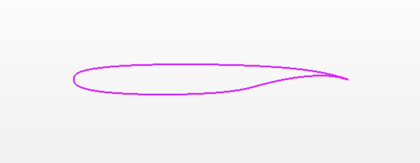
The geometries of the airfoils are given in separate files as a set of coordinates. These data sets can be imported in Geometry -> 3D-CAD Models as follows:
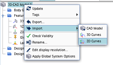
After selecting the file to be imported, in the pop-up window select Import as 2D spline and Close the curve.
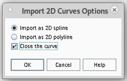
A new skech is generated including the imported wing geometry.
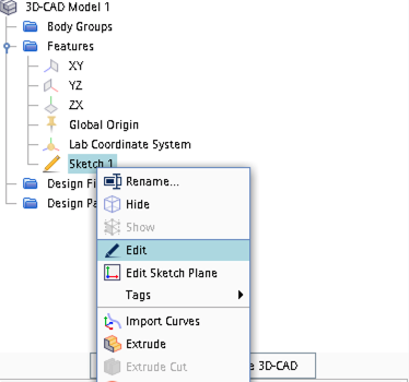
To Finalize the domain definition, right click Sketch 1 and click on Edit in the menu.
CFD guidelines
Some general guidelines for the simulation:
- Don't forget to set the reference pressure to zero:
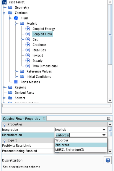
Continua -> Fluid -> Reference Values -> Reference Pressure- In your project, you should investigate the performance of different numerical schemes. The numerical scheme is modified under
Continua -> Fluid -> Models -> Coupled Flow. Note, in case you have not renamed the physics entry underContinua, the default name isPhysics 1.
- Some of the cases, or at least some of the operation conditions for some cases, will have convergence problems due to flow instabilities. In case you get that type of solver behavior, try to find another convergence criterion by for example measuring forces or massflow. You may also consider updating the mesh as it is crucial to resolve important flow features to reach convergence.
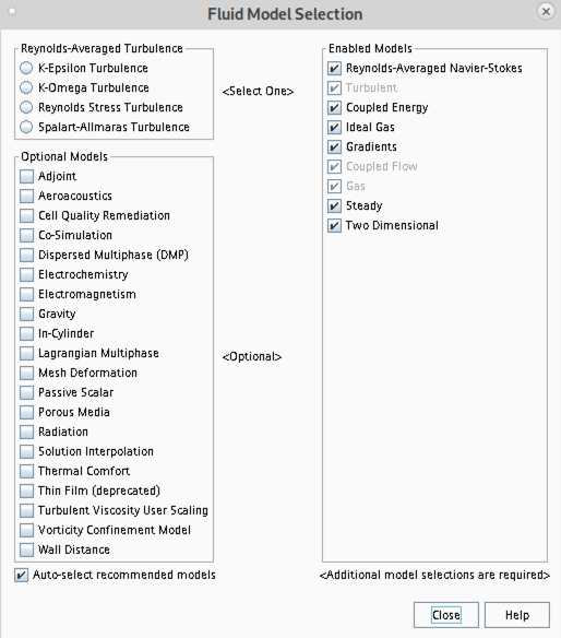
- Some of the cases should be simulated using a viscous solver. Choose
Turbulentinstead ofInviscidwhen you select models and then select an appropriate turbulence model.
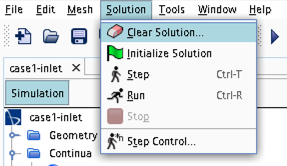
- In case you would like to start your simulation from scratch, the flow field can be reset as indicated in the picture below (don't forget to initialize the flow field after the reset).
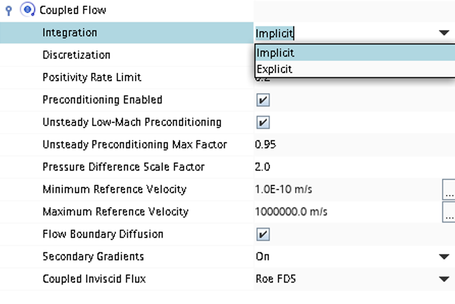
- Time stepping approach (implicit/explicit) is selected under
Continua -> Fluid -> Models -> Coupled Flow
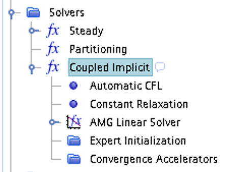
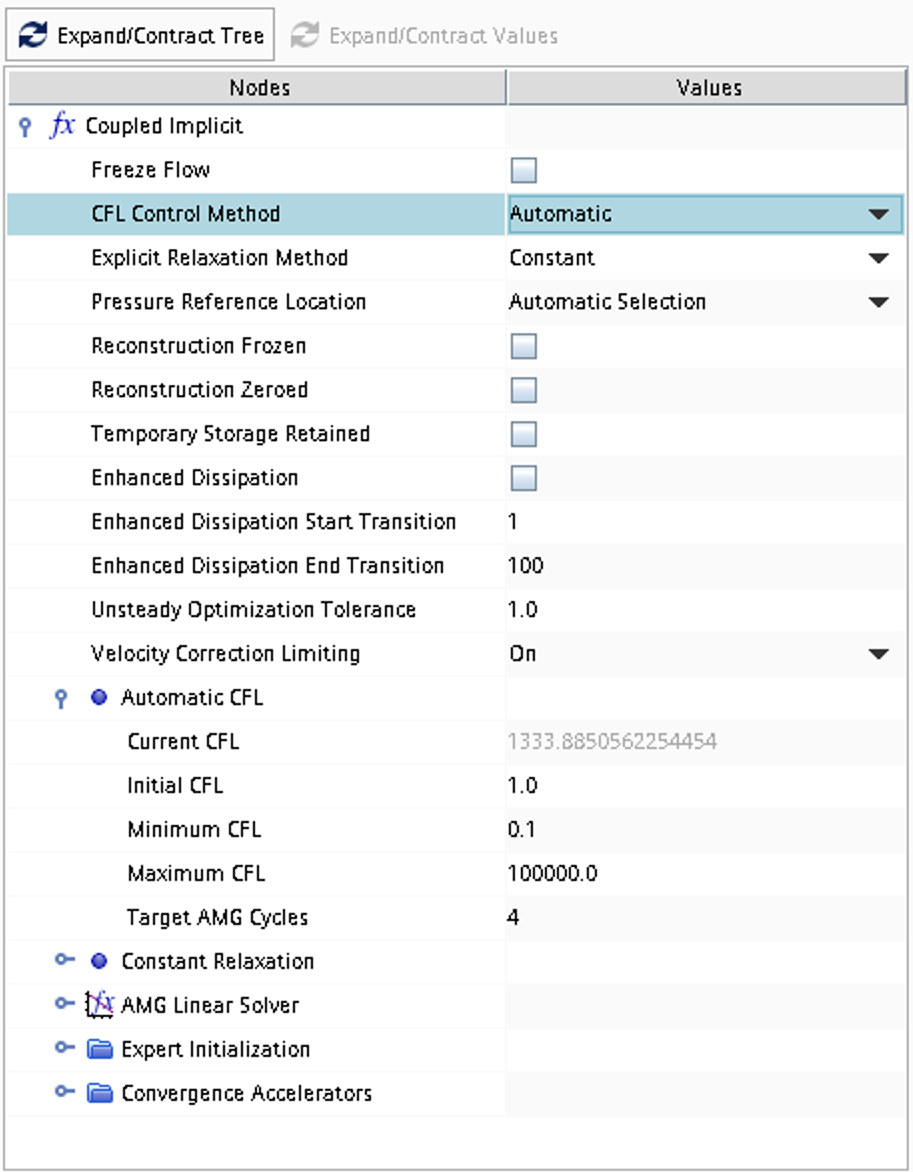
- CFL number and other solver settings are found under
Solver -> Coupled Implicit(orSolver -> Coupled Explicit)