Case 4
Inviscid compressible over-expanded nozzle flow (steady-state)
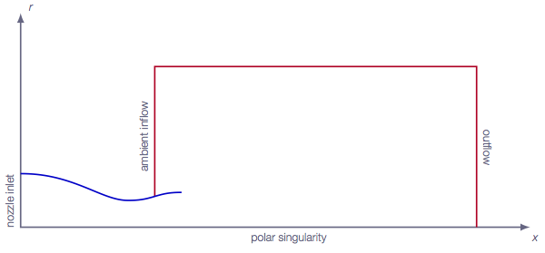
 Inviscid compressible flow in two space dimensions (axial coordinate \(x\) and radial coordinate \(r\)) and time is assumed. A geometry according to the picture below is defined and the problem consists of computing numerically the 2D axi-symmetric steady-state flow including any possible shocks outside of the nozzle.
Literature review
Suggested search topics
- Shock diamonds (shock-cell structure)
- Geometry effects on nozzle flow
Specifications
- Area ratio between nozzle inflow and throat: 4.0
- Area ratio between nozzle outflow and throat: 1.69
- The geometry of the nozzle contour is arbitrary but should be smooth on the inside
- For all operating conditions, ideal gas is assumed
| operating condition 1 | |
| Nozzle inflow | \(p_o=1.028\) bar, \(T_o=300\) K, velocity in \(x\)-direction |
| Ambient inflow | \(p_o=1.007\) bar, \(T_o=300\) K, velocity in \(x\)-direction |
| Outflow | \(p=1.0\) bar |
| operating condition 2 | |
| Nozzle inflow | \(p_o=1.186\) bar, \(T_o=300\) K, velocity in \(x\)-direction |
| Ambient inflow | \(p_o=1.007\) bar, \(T_o=300\) K, velocity in \(x\)-direction |
| Outflow | \(p=1.0\) bar |
| operating condition 3 | |
| Nozzle inflow | \(p_o=1.524\) bar, \(T_o=300\) K, velocity in \(x\)-direction |
| Ambient inflow | \(p_o=1.007\) bar, \(T_o=300\) K, velocity in \(x\)-direction |
| Outflow | \(p=1.0\) bar |
| operating condition 4 | |
| Nozzle inflow | \(p_o=1.893\) bar, \(T_o=300\) K, velocity in \(x\)-direction |
| Ambient inflow | \(p_o=1.007\) bar, \(T_o=300\) K, velocity in \(x\)-direction |
| Outflow | \(p=1.0\) bar |
| operating condition 5 | |
| Nozzle inflow | \(p_o=2.425\) bar, \(T_o=300\) K, velocity in \(x\)-direction |
| Ambient inflow | \(p_o=1.007\) bar, \(T_o=300\) K, velocity in \(x\)-direction |
| Outflow | \(p=1.0\) bar |
| operating condition 6 | |
| Nozzle inflow | \(p_o=3.182\) bar, \(T_o=300\) K, velocity in \(x\)-direction |
| Ambient inflow | \(p_o=1.007\) bar, \(T_o=300\) K, velocity in \(x\)-direction |
| Outflow | \(p=1.0\) bar |
| operating condition 7 | |
| Nozzle inflow | \(p_o=3.912\) bar, \(T_o=300\) K, velocity in \(x\)-direction |
| Ambient inflow | \(p_o=1.007\) bar, \(T_o=300\) K, velocity in \(x\)-direction |
| Outflow | \(p=1.0\) bar |
| operating condition 8 | |
| Nozzle inflow | \(p_o=5.868\) bar, \(T_o=300\) K, velocity in \(x\)-direction |
| Ambient inflow | \(p_o=1.007\) bar, \(T_o=300\) K, velocity in \(x\)-direction |
| Outflow | \(p=1.0\) bar |
| operating condition 9 | |
| Nozzle inflow | \(p_o=7.824\) bar, \(T_o=300\) K, velocity in \(x\)-direction |
| Ambient inflow | \(p_o=1.007\) bar, \(T_o=300\) K, velocity in \(x\)-direction |
| Outflow | \(p=1.0\) bar |
Expected results and presentation
The solutions obtained should be presented in the form of density/pressure/Mach contour plots, showing any special features in the flow such as shocks.
Based on the Mach contour plots for the different operating conditions, describe what happens with the flow as the ratio between inflow and outflow pressures increases. If a shock appears, what happens with its position and strength?
For the internal shock cases, compare shock locations with quasi-one-dimensional theory, i.e., make an estimate of the shock location analytically and compare with the shock location predicted by STAR-CCM+.
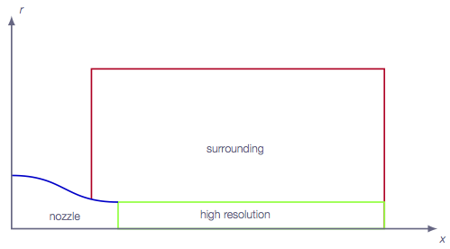
Grid generation guidelines
There should not be any large jump in cell sizes anywhere. The changes in cell size must be smooth otherwise you might run into problems with convergence.
The jet emanating from the nozzle and the divergent section of the nozzle are the most important parts to resolve really well. Make sure that the high-resolution area is able to resolve oblique shocks that may appear for some of the operating conditions.
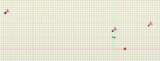
The nozzle contour can be generated using the spline functionality in the STAR-CCM+ sketch tool. Start by making three points using the Create point tool.
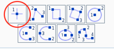
Adjust the coordinates according to the specifications above. The length of the nozzle is not specified but choose a length that makes it possible to generate a smooth curve from inlet to outlet. Then right click on each of the three points and click Apply Fixation Constraint. This will make sure that the spline generation tool does not modify the location of these coordinates later.
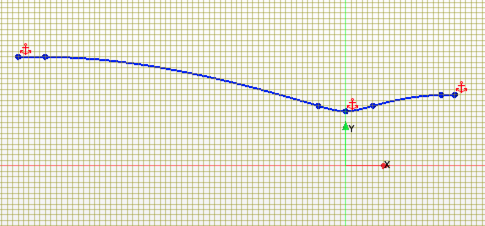
Now, use the Create Spline tool to generate the nozzle contour.
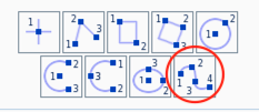
Select the nozzle inlet coordinate as the first point on the spline curve, then select two points between the nozzle inlet and the nozzle throat (these points can be moved later). Select the nozzle throat coordinate as the fourth point and then two additional points between the throat and the nozzle exit. Finally select the nozzle outlet coordinate as the end point. Press esc on your keyboard to exit the spline tool. Move the four control points such that the nozzle contour looks smooth. OBS! make sure that the throat area is the minimum area in the nozzle.
CFD guidelines
It is recommended that the initial solution for operating condition 1 is set from ambient inflow conditions, i.e., with a velocity in the \(x\)-direction. The steady-state solution obtained for operating condition 1 should then be used as initial solution for operating condition 2, the steady-state solution obtained for operating condition 2 should be used as initial solution for operating condition 3 and so on. This minimizes potential difficulties due to too large mismatches between initial solutions and boundary conditions. This means that when one operating condition is converged, the nozzle inlet pressure can be updated such that it represents the next operation condition and then the solver is started again. Make a copy of the converged operation condition in case you would like to go back. In some cases, the jump in pressure ratio between two operation conditions in the table is too high and the solver might diverge. If that is the case, make one or several intermediate simulations (smaller steps in total pressure).
- The solver mode should not be
Two dimensional, selectAxisymmetricinstead. In caseTwo dimensionalis selected by default, deselect it and selectAxisymmetric. - The polar singularity boundary condition should be set as follows:
Type: Axis
Some general guidelines for the simulation:
- Don't forget to set the reference pressure to zero:
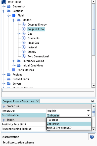
Continua -> Fluid -> Reference Values -> Reference Pressure- In your project, you should investigate the performance of different numerical schemes. The numerical scheme is modified under
Continua -> Fluid -> Models -> Coupled Flow. Note, in case you have not renamed the physics entry underContinua, the default name isPhysics 1.
- Some of the cases, or at least some of the operation conditions for some cases, will have convergence problems due to flow instabilities. In case you get that type of solver behavior, try to find another convergence criterion by for example measuring forces or massflow. You may also consider updating the mesh as it is crucial to resolve important flow features to reach convergence.
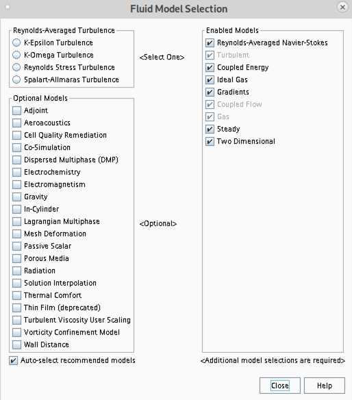
- Some of the cases should be simulated using a viscous solver. Choose
Turbulentinstead ofInviscidwhen you select models and then select an appropriate turbulence model.
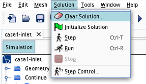
- In case you would like to start your simulation from scratch, the flow field can be reset as indicated in the picture below (don't forget to initialize the flow field after the reset).
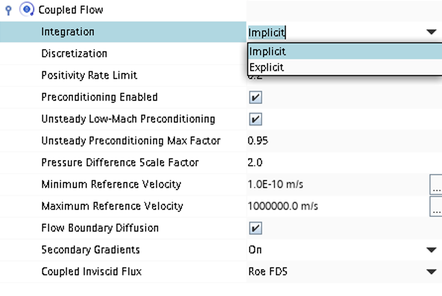
- Time stepping approach (implicit/explicit) is selected under
Continua -> Fluid -> Models -> Coupled Flow
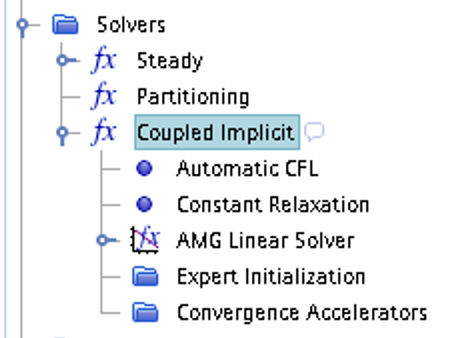
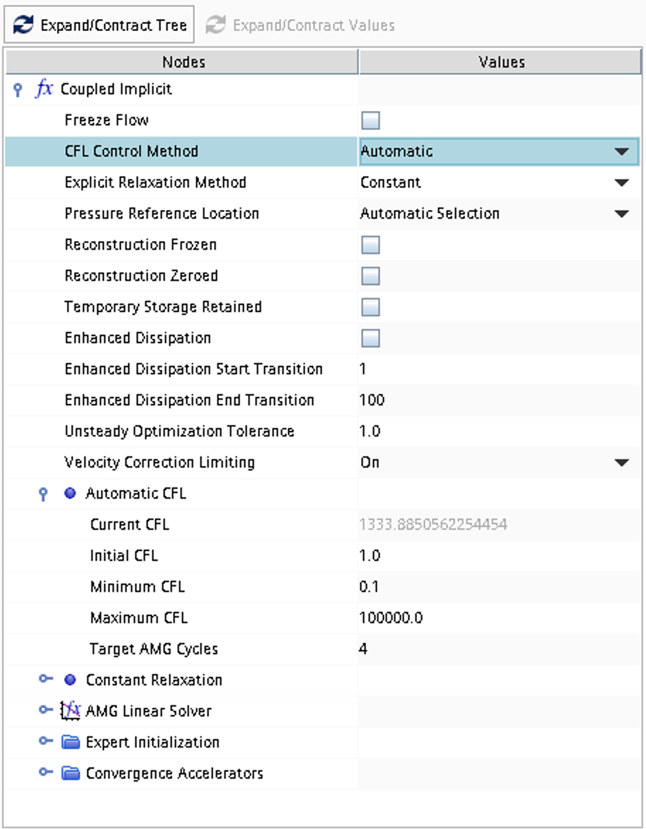
- CFL number and other solver settings are found under
Solver -> Coupled Implicit(orSolver -> Coupled Explicit)