One-Dimensional Flow

---

Overview

The third chapter in the book deals with flows that can be assumed to be one dimensional, i.e. flow quantities will only vary in one direction. Although this may seem to be of very limited use, the theory covered and equations derived in this section will be of great help in the coming chapters. The specific model problems analyzed in detail in chapter three are: normal shocks, one-dimensional flow with heat addition, and one-dimensional flow with friction.

Online Flow Calculator

Sections of the online flow calculator for compressible flow problems CFLOW related to this chapter:

• Section 1: Gas Relations
• Section 2: Total Flow Properties
• Section 3: Normal Shock Relations
• Section 4: 1D Flow with Heat Addition
• Section 5: 1D Flow with Friction

The CFLOW finite-volume quasi-1D solver can also be used to study the problems in this chapter.

Chapter Roadmap

Sections

3.2 One-dimensional Flow Equations

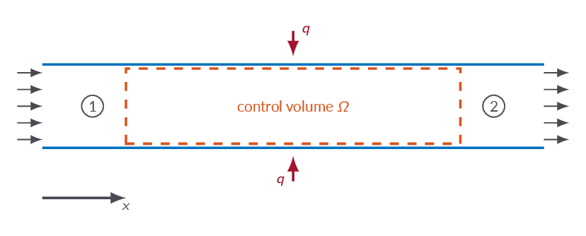
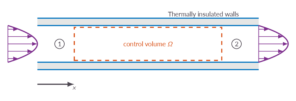
The one dimensional flow equations are derived starting from the conservation equations on integral form introduced in Chapter 2. With variation of flow quantities in one direction only, a simplified set of governing equations is derived using a control volume approach.

conservation of mass

$$ \rho_1 u_1 = \rho_2 u_2$$

conservation of momentum

$$ p_1 +\rho_1 u_1^2 = p_2 + \rho_2 u_2^2 $$

conservation of energy

$$ h_1 +\frac{u_1^2}{2} = h_2 + \frac{u_2^2}{2} $$

3.3 Speed of Sound and Mach Number

Using the above derived equations and choosing a control volume such that it includes the wave front of an acoustic wave the speed of sound is investigated. Using the fact that an acoustic wave is a very weak wave we can make assumptions about changes in flow quantities and losses that leads us to a relation between the speed of sound and the compressibility

$$ a^2=\left(\frac{\partial p}{\partial \rho}\right)_s $$

Finally, by assuming that we can treat the gas as calorically perfect, we end up with the following relation between speed of sound and temperature

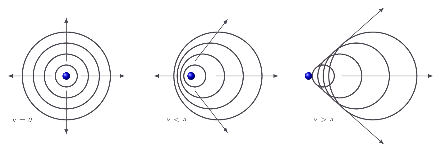
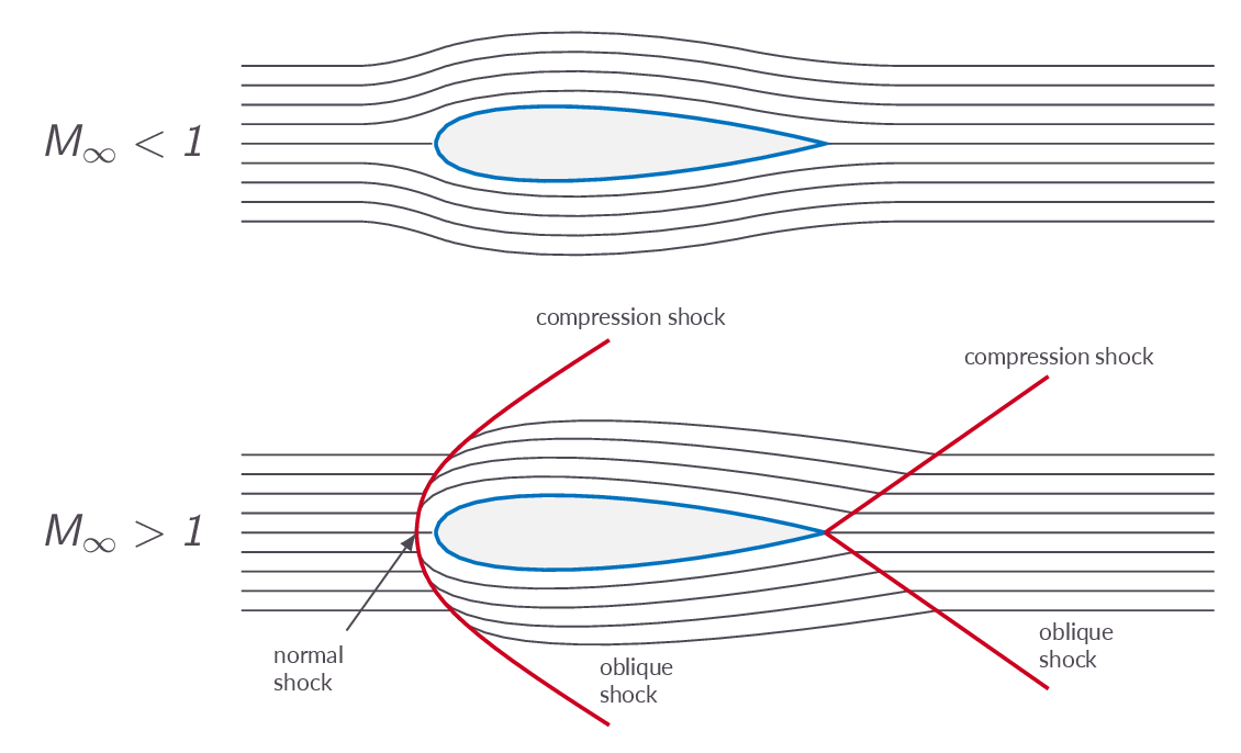
$$ a=\sqrt{\gamma RT} $$

From the relation above, it is obvious that the local speed of sound is related to the temperature of the flow, which in turn is a measure of the motion of elementary particles (atoms and/or molecules) of the fluid at a specific location. This stems from the fact that sound waves are propagated via interaction of these elementary particles. Since information in a flow is propagated via molecular interaction the relation between the speed at which this information is conveyed and the speed of the flow has important physical implications. Figure 1 compares three sound wave patterns generated by a a beacon. In the left picture, the sound transmitter is stationary and thus the acoustic waves are centered around the transmitter. In the middle image, the transmitter is moving to the left at a speed less than the speed of sound and thus the transmitter will always be within all sound wave circles but it will be off-centered with a bias in the direction that the transmitter is moving. In the right image the transmitter is moving faster than the speed of sound and thus it will always be located outside of all acoustic waves. In a supersonic flow, no information can travel upstream and therefore there is no way for the flow to adjust to downstream obstacles. This is compensated for by the introduction of shocks in the flow. Over a shock flow properties changes discontinuity. An example is given in Figure 2 below.

3.4 Some Conveniently Defined Flow Parameters

This section introduces total and critical flow properties. The total properties represent the condition that we would have if we could slow the flow down to zero velocity isentropically (without losses). The critical properties represent the condition that we would have if we could accelerate or decelerate the flow adiabatically to sonic conditions. It is important to understand that the it is not required that the flow is isentropic to be able to obtain the total conditions, e.g. total pressure (\(p_o\)) and total temperature (\(T_o\)), it is the imaginary process of slowing the fluid down to zero velocity that is isentropic. However, if the flow is isentropic, the stagnation properties (total conditions) will be constants in the flow and can be used as reference states in calculations. In fact, total temperature (\(T_o\)) is constant in the flow as long as the flow is adiabatic (no heat exchange) but constant total pressure (\(p_o\)) requires isentropic flow (adiabatic and reversible). Changes in total pressure are often used as a measure of flow losses (ireversibillities in the flow). Since the imaginary process used to reach total flow conditions is, by definition, isentropic, the isenropic relations introduced in Chapter 1 can be used to get relations between stagnation flow properties. The same is true for the critical conditions if the process is reversible.

The characteristic Mach number is defined as the Mach number calculated with the local velocity and the speed of sound at sonic conditions

$$M^\ast=\dfrac{V}{a^\ast}$$

It can be shown that the characteristic mach number, although it differs from the Mach number in value, behaves as the Mach number. This fact is used in the analysis of the normal-shock relations derived later.

3.5 Alternative Form of the Energy Equation

Using the definition of speed of sound for calorically perfect gases and the relations derived in the previous section one can rewrite the energy equation to obtain ratios of total and local flow properties and ratios of characteristics and local flow properties, respectively.

Total enthalpy is defined as

$$h_o=h+\dfrac{1}{2}V^2$$

For calorically perfect gases we have

$$h=C_p T$$ $$C_p T_o = C_p T + \dfrac{1}{2}V^2$$ $$\dfrac{T_o}{T}=1+\dfrac{1}{2}\dfrac{V^2}{C_p T}$$

Now use the relation between \(C_p\), \(\gamma\), and \(R\) introduced in Chapter 1 $$C_p = \dfrac{\gamma R}{\gamma - 1}$$ $$\dfrac{T_o}{T}=1+\dfrac{1}{2}\left(\dfrac{1}{\gamma-1}\right)\dfrac{V^2}{\gamma R T}$$

Since \(a^2=\gamma R T\) for a calorically perfect gas we get

$$\dfrac{T_o}{T}=1+\dfrac{1}{2}\left(\dfrac{1}{\gamma-1}\right)M^2$$

3.6 Normal Shock Relations

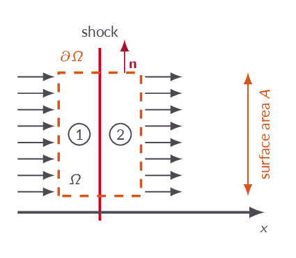
Applying the control volume approach to a one-dimensional flow with a normal shock situated within the control volume leads to the normal shock relations. The normal shock relations are derived starting from the adiabatic flow equations (since there will be no heat exchange inside the shock) and results in a set of expressions relating ratios of flow quantities from regions upstream of the shock and corresponding properties on the downstream side to the upstream Mach number. The relation between the characteristics Mach number on the upstream side \(M^*_1\) and the characteristic Mach number on the downstream side of the normal shock \(M^*_2\) tells us that behind a normal shock the flow is always subsonic.

The balance analysis of the control volume with the shock inside gives as a result the so-called Prandtl relation.

$${a^\ast}^2=u_1u_2$$

where indices 1 and 2 denotes the upstream and downstream flow states, respectively. Prandlt's relation can be rewritten as

$$M_1^\ast=\dfrac{1}{M_2^\ast}$$

which effectively shows that if the Mach number upstream of the shock is greater than one, the downstream Mach number must be less than one and vice versa. We can also see that a sonic upstream flow (\(M_1=1.0\)) gives sonic flow downstream of the shock. So, apparently the relation as such holds for both supersonic and subsonic upstream flow mathematically. The question is if it is also physically correct. For a supersonic upstream flow we will get a discontinuous compression and if the flow upstream of the control volume is subsonic we will instead get a discontinuous expansion inside the control volume but, again, is this physically correct. We will get the answer by analyzing the entropy change over the control volume.

Analyzing the energy equation and the second law of thermodynamics shows that there is a direct relation between entropy increase and total pressure drop.

$$s_2-s_1=C_p\ln\dfrac{T_2}{T_1}-R\ln\dfrac{p_2}{p_1}$$ $$s_2-s_1=C_p\ln\dfrac{T_2}{T_{o_2}}\dfrac{T_{o_1}}{T_1}\dfrac{T_{o_2}}{T_{o_1}}-R\ln\dfrac{p_2}{p_{o_2}}\dfrac{p_{o_1}}{p_1}\dfrac{p_{o_2}}{p_{o_1}}$$

using the isentropic relations we get

$$s_2-s_1=C_p\ln\dfrac{T_{o_2}}{T_{o_1}}-R\ln\dfrac{p_{o_2}}{p_{o_1}}$$

and since the process is adiabatic and thus \(T_{o_2}=T_{o_1}\) the change in entropy is directly related to the change in total pressure as

$$s_2-s_1=-R\ln\dfrac{p_{o_2}}{p_{o_1}}$$

or

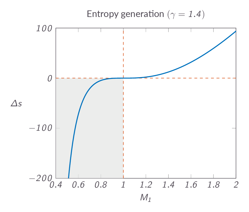
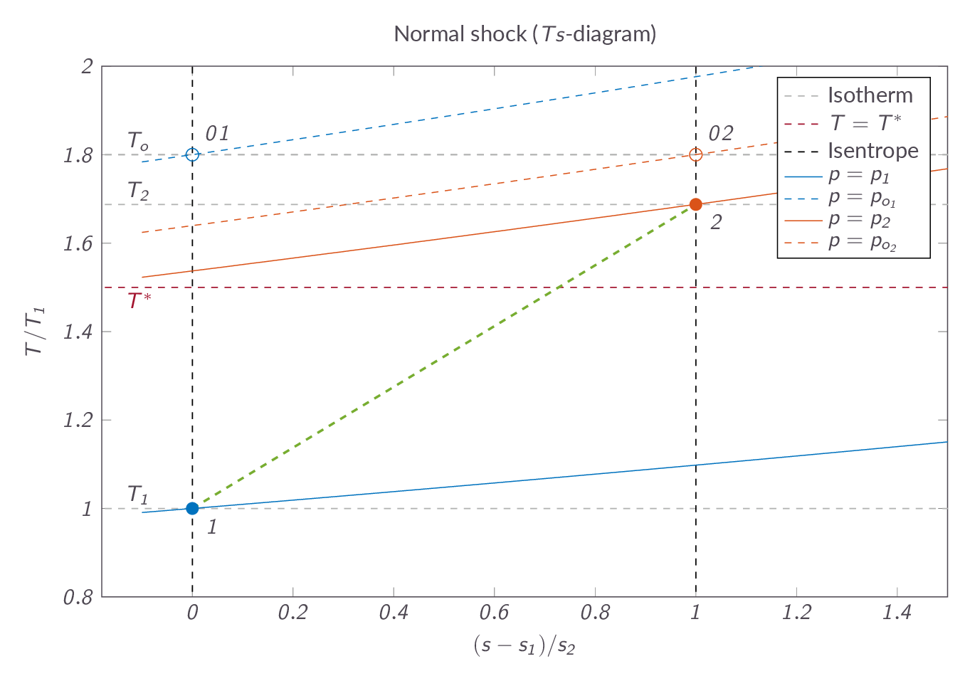
$$\dfrac{p_{o_2}}{p_{o_1}}=e^{-(s_2-s_1)/R}$$

The figure below shows the entropy change over a normal shock. As can be seen in the figure, a subsonic upstream Mach number leads to a reduction of entropy, which once and for all rules out all such solutions as non-physical and thus the question about the upstream conditions can now be considered answered. This in turn implies that the Mach number downstream of a normal shock will always be subsonic, which can be seen in Figure XX below.

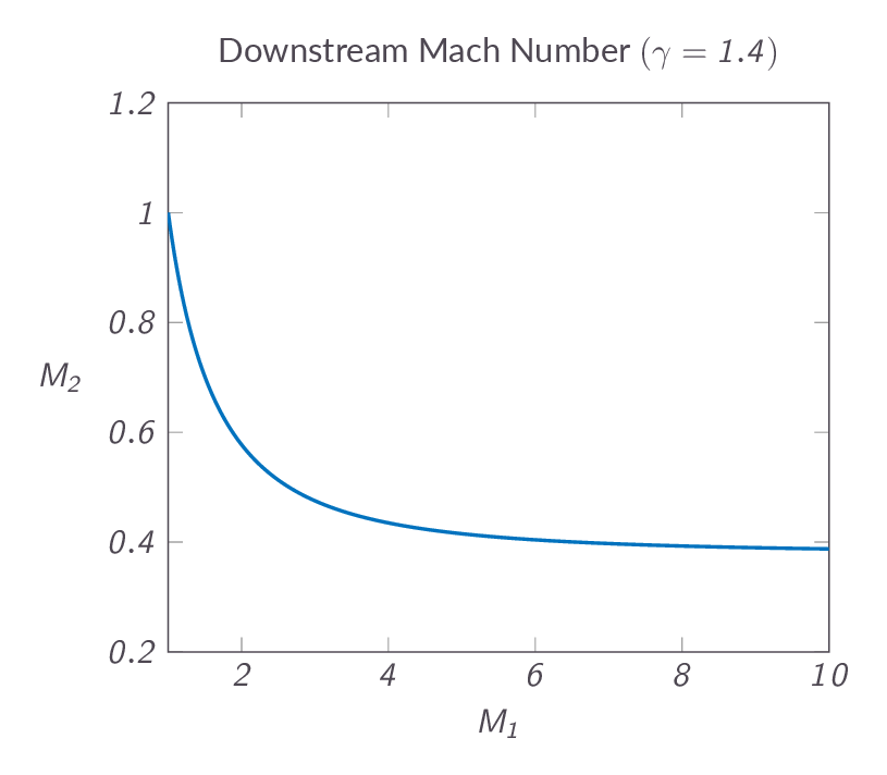
The downstream Mach number is given as a function of the upstream Mach number by the following relation

$$M_2^2=\dfrac{1+\dfrac{1}{2}(\gamma-1)M_1^2}{\gamma M_1^2-\dfrac{1}{2}(\gamma-1)}$$

Analyzing the relation, one can see that the downstream Mach number approaches \(\sqrt{(\gamma-1)/2\gamma}\) as the upstream Mach number approaches infinity.

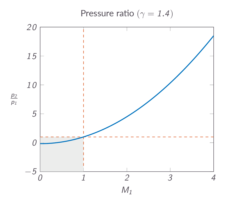
The pressure ratio over the normal shock is given by

$$\dfrac{p_2}{p_1}=1+\dfrac{2\gamma}{\gamma+1}\left(M_1^2-1\right)$$

Figure XX below shows that the pressure must increase over the shock and thus the shock is a discontinuous compression process.

Now, one question remains. How come that we by analyzing the control volume using the upstream and downstream states get the normal shock relations. There is no way that the governing equations could have known about the fact that we assumed that there would be a shock inside of the control volume, or is it? The answer is that we have assumed that there will be a change in flow properties from upstream to downstream. We have further assumed that the flow is adiabatic (we are using the adiabatic energy equation) so there is no heat exchange. We are, however, allowing for irreversibilities in the flow. The only way to accomplish a change in flow properties under those constraints is a formation of a normal shock (a discontinuity in flow properties - a sudden flow compression) between station 1 and station 2.

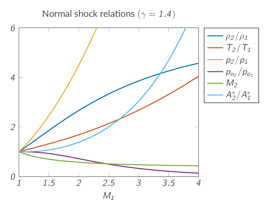
Figure XX below shows how different flow properties change over a normal shock as a function of upstream Mach number.

3.7 The Hugoniot Equation

The Hugoniot equation is an alternative normal shock relation based on thermodynamic quantities only.

The Hugoniot equation is derived from the governing equations and relates the change in energy to the change in pressure and specific volume

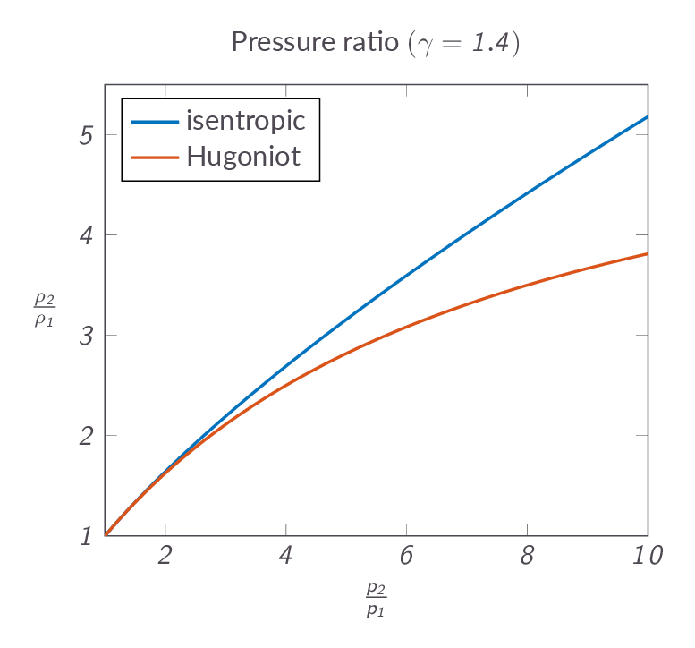
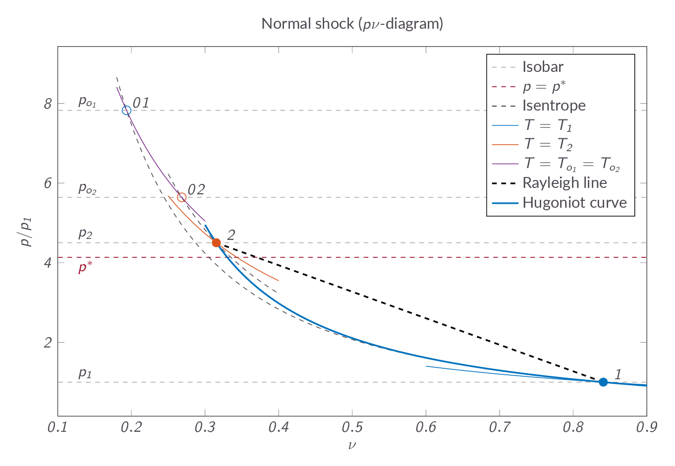
$$e_2-e_1=\dfrac{p_2+p_1}{2}(\nu_1-\nu_2)$$

To give an idea about how the normal shock relates to an isentropic compression (a flow compression process without losses) the change in flow density as a function of pressure ratio is compared in Figure XX below. One can see that the normal-shock compression is more effective but less efficient than the corresponding isentropic process.

Introducing C as the massflow per unit area (which is a constant)

$$\rho_1 u_1 = \rho_2 u_2 = C$$

Inserted into the momentum equation this gives

$$p_1+\dfrac{C^2}{\rho_1}=p_2+\dfrac{C^2}{\rho_2}$$

or

$$\dfrac{p_2-p_1}{\nu_2-\nu_1}=-C^2$$

which implies that all possible solutions to the governing equations must be located on a line in \(p\nu\)-space (the so-called Rayleigh line). If we add the Hugoniot relation to this we will find that there are two possible solutions, the upstream condition and the condition downstream of the normal shock and the flow cannot be in any of the intermediate stages. The normal-process is a so-called wave solution to the governing equations where the flow state must jump directly from one flow state to another without passing the intermediate conditions. If we add heat or friction to the problem we will instead get continuous solutions as we will see in the following sections. Figures XX and YY shows a normal shock process in a \(p\nu\)- and \(Ts\)-diagram, respectively. Note that the flow passes the characteristic conditions as it is going through the shock, which means that the flow goes from supersonic to subsonic.

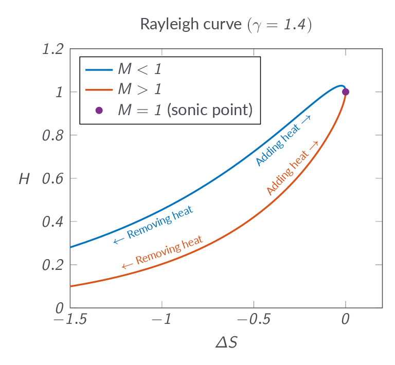
3.8 One-Dimensional Flow with Heat Addition

With heat addition in our control volume we end up with a heat addition term in the energy equation. This means that in contrast to the normal shock case we are, obviously, no longer using the adiabatic energy equation, which does have significant effects on the physical processes and the consequently outcome of the control volume analysis. The main difference is that since heat is considered to be added continuously over the axial extent of the control volume (since we are still studying one-dimensional problems), the process and thus the change of physical properties will also be continuous as we move through the control volume. Hence one-dimensional flow with heat addition is not a problem with a wave solution, it is a problem with a continuous solution.

Analyzing the energy equation with added heat, it is obvious that a direct effect of the heat addition is an increase of total temperature.

$$h_1+\dfrac{1}{2}u_1^2+q=h_2+\dfrac{1}{2}u_2^2$$ $$C_p T_1+\dfrac{1}{2}u_1^2+q=C_p T_2+\dfrac{1}{2}u_2^2$$ $$q=\left(C_p T_2+\dfrac{1}{2}u_2^2\right)-\left(C_p T_1+\dfrac{1}{2}u_1^2\right)$$ $$ q=C_p(T_{o2}-T_{o1}) $$

It is shown that adding heat will bring the flow Mach number closer to unity. If the flow is subsonic, adding heat will increase the flow Mach number until the flow reaches sonic conditions. After that adding more heat will not be possible without changing the inflow conditions. For a supersonic flow, adding heat will lower the Mach number until the flow is sonic.

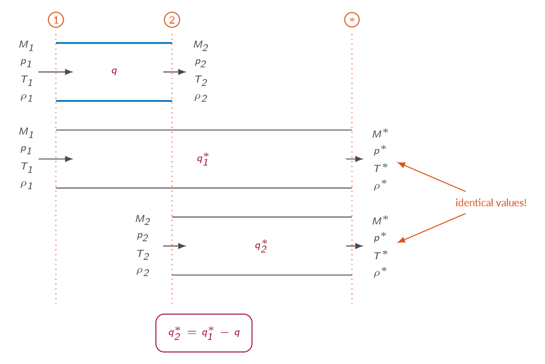
In this section a new set of starred flow quantities are introduced. In this case the star denotes the flow properties that we would get if enough heat was added to reach sonic conditions. The starred quantities are constants in a given flow and can thus be used as a reference state when solving problems.

3.9 One-Dimensional Flow with Friction

The governing equations for one-dimensional flow with friction are derived. The introduction of friction gives results in the addition of an integral in the momentum equation and the equations are transformed to differential form. In the same way as adding heat lead to changed flow properties, the effect of the friction will be that the Mach number of a subsonic flow will be increased with increased pipe length until sonic conditions are reached and the Mach number of a supersonic flow will be decreased.

A new set of starred quantities are introduced. For one-dimensional flow with friction, the starred flow properties represent the condition that we would have if the pipe was long enough to reach sonic conditions at the end. When sonic conditions are reached \(L=L^*\), the pipe cannot be made longer without modifying the inlet boundary conditions.

---

Study Guide

The questions below are intended as a "study guide" and may be helpful when reading the text book.

Auxiliary Relations

Stationary Normal Shock in One-Dimensional Flow

One-Dimensional Flow with Heat Addition

One-Dimensional Flow with Friction