Introduction
 In this exercise, you will investigate flow inside a convergent divergent nozzle and the unsteady wave motion in a shock tube using the Q1D solver available in CFLOW. In total, you will investigate four flow cases of which three are nozzle flows and one is the flow in a shock tube.
OBS Read chapters 5-7 in the course book before starting with the exercise!
When you have done the assignment, you should write a short report and hand in for assessment of this course element (instructions at the bottom of this page).
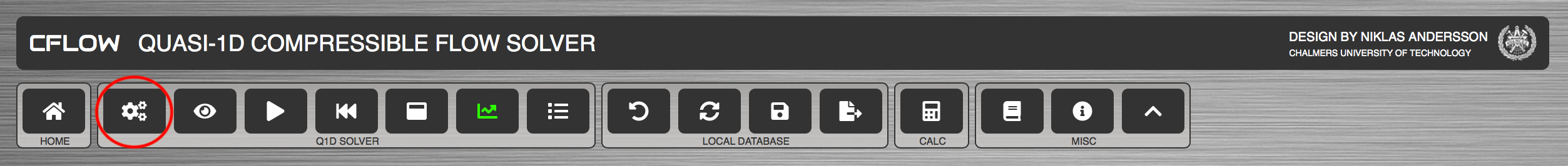
The CFLOW solver is a solver for simulation of compressible flows based on an explicit time-marching finite-volume-method (FVM) approach for which you can find a thorough description in the lectures on time-marching methods (Lectures 13 and 14). In order to be able to solve the tasks, you will have to make changes to the solver settings in accordance with the task description such as tube geometry, number of cells, number of time steps, boundary conditions, and initial flow properties. In order for the solver to run in a stable manner, you will also need to make changes to the solver numerics settings in some of the cases. In cases with steep gradients or discontinuities, extra damping will be needed. The extra damping is activated in the Numerics section. Pressure damping is used for shocks and density damping is for cases with steep temperature gradients.
Note that for compressible flows, the CFL-number is defined as:
$$CFL=\frac{\Delta t(c+|u|)}{\Delta x}$$
where \(\Delta t\) is the time step size, \(c\) is the speed of sound, \(u\) is the fluid velocity, and \(\Delta x\) is the local cell size. Since the solver uses explicit time marching, it is important that the CFL-number is below unity, otherwise the computation may diverge. You can find more details on the numerics of compressible flow solvers in the lecture notes on time-marching methods.
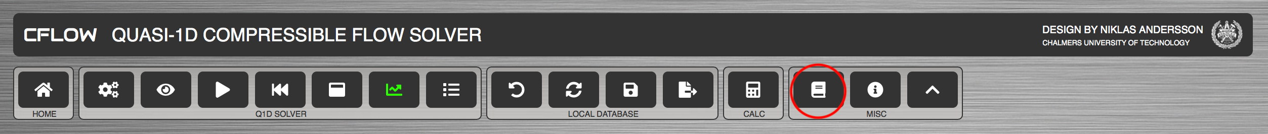
Detailed description of the solver settings and solver functionality can be found in the solver manual.
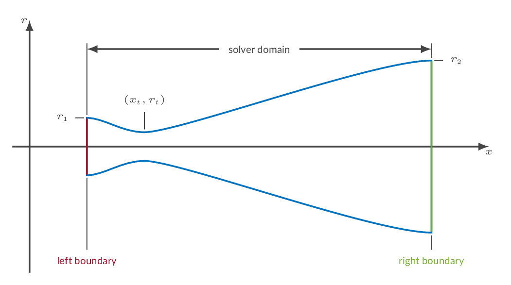
Computational Domain
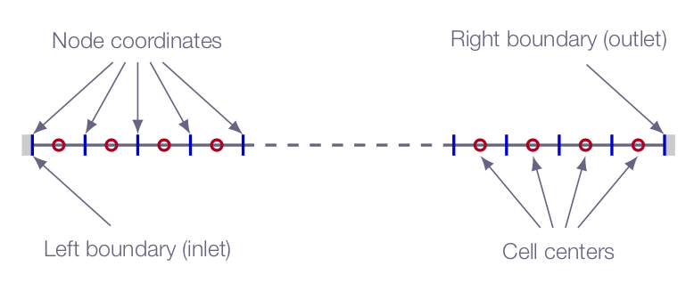
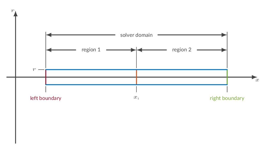
The figure below shows a schematic representation of the computational domain in CFLOW. Note that the solver is of finite-volume-method (FVM) type, which means that it solves for cell averages of flow properties.
Convergence
The convergence history is visualized in the solver log. Depending on task, the number of iterations needed in order to reach convergence will vary. In case the solver is not converged when the specified number of iterations are completed, increase the number of iterations and restart the solver.
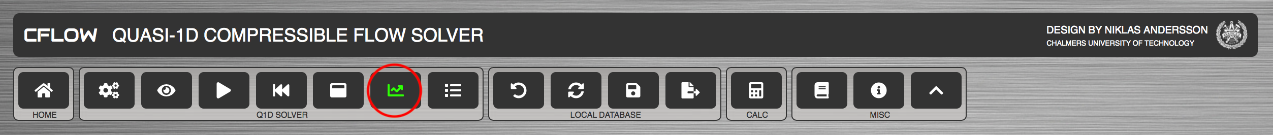
Postprocessing
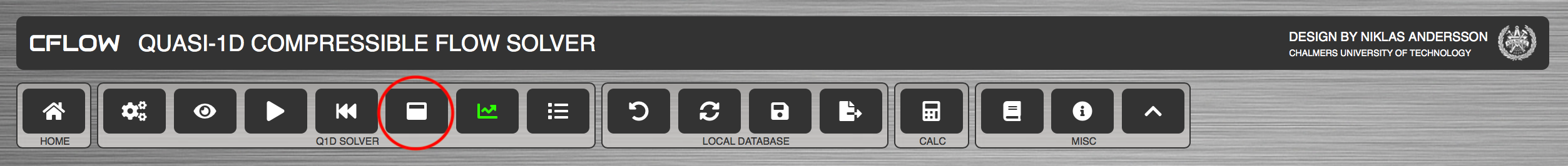
CFLOW will produce graphs of \(\rho\), \(u\), \(p\), \(T\), \(M\), \(p_o\), and \(T_o\) for each obtained solution. Study the graphs and make sure that you can explain what you see.
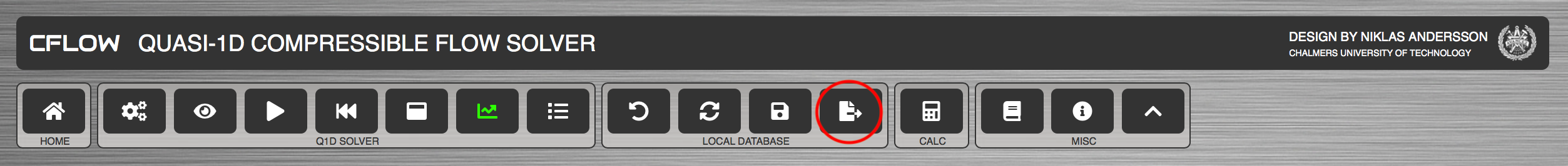
Export
When done with one of the tasks below, save the CFLOW state to a JavaScript data base file (JSON) using the export functionality. The file can later be used to restore the solver state and should be submitted in Canvas along with the report.
The following tasks should be solved both analytically and numerically. Note that in order to be able to apply the correct boundary conditions in the numerical simulations, you will need to solve the problems analytically first!
Task 1 - Quasi-1D simulation of the flow in a convergent-divergent nozzle
Task 1a - nozzle flow with internal shock
In this task you will simulate air flow through a convergent divergent nozzle. The exit and throat areas of the nozzle are 0.5 m\(^2\) and 0.25 m\(^2\), respectively. The nozzle inlet area can be set to 0.3 m\(^2\). The inlet reservoir pressure and temperature (total pressure and total temperature upstream of the nozzle inlet) are 1.0 atm and 288 K, respectively. In this first task, the exit static pressure (back pressure) is 0.6 atm. Setup the CFLOW solver using the recommended settings below and compare the results with your calculations. Is the shock location correct?
Remember to export the solver state to a JSON-file when you are done with the task.
| Geometry definition |
| pipe type |
convergent divergent nozzle |
| left-end coordinate |
0.0 |
| right-end coordinate |
1.0 m |
| throat coordinate |
0.33 m |
| left end cross section (area) |
0.3 m^2 |
| right end cross section (area) |
0.5 m^2 |
| throat cross section (area) |
0.25 m^2 |
| Mesh properties |
| Number of cells |
100 (refine later if needed) |
| Cell spacing |
uniform mesh |
| Numerics |
| Artificial damping (shocks) |
0.5 (there will be a shock in the nozzle) |
| Artificial damping (temperature) |
0 - not needed (no steep temperature gradients) |
| Time-stepping mode |
local time stepping |
| CFL number |
0.9 |
| Run parameters |
| Number of time steps |
with the specified settings the solver should converge within 3000 iterations - check convergence after completing the simulation though and add more iterations if needed. If you increased the cell count, you will most likely need to increase the number of iterations to get a converged solution. |
| Gas properties |
|
use the default settings for air |
| Initial flow field |
| Initialization mode |
constant values |
| Flow field data |
use the exit conditions as initial flow |
| Boundary conditions |
| Left-end boundary |
subsonic inflow |
| Right-end boundary |
subsonic outflow |
Task 1b - choked subsonic nozzle flow
In this task you will simulate air flow through the same convergent divergent nozzle as in Task 1a but in this case the critical condition should be simulated (choked subsonic flow). Calculate the exit conditions corresponding to choked nozzle flow and set up the CFLOW according to the recommendations given below. Do the results look as expected? Are there any significant difference from the analytical solution?
Remember to export the solver state to a JSON-file when you are done with the task.
| Geometry definition |
| pipe type |
convergent divergent nozzle |
| left-end coordinate |
0.0 |
| right-end coordinate |
1.0 m |
| throat coordinate |
0.33 m |
| left end cross section (area) |
0.3 m^2 |
| right end cross section (area) |
0.5 m^2 |
| throat cross section (area) |
0.25 m^2 |
| Mesh properties |
| Number of cells |
100 (refine later if needed) |
| Cell spacing |
uniform mesh |
| Numerics |
| Artificial damping (shocks) |
0.5 (even though there should not be any shocks in the solution, shocks may appear during the iterations depending on solver settings) |
| Artificial damping (temperature) |
0 - not needed (no steep temperature gradients) |
| Time-stepping mode |
local time stepping |
| CFL number |
0.9 |
| Run parameters |
| Number of time steps |
with the specified settings the solver should converge within 85000 iterations - check convergence after completing the simulation though and add more iterations if needed. If you increased the cell count, you will most likely need to increase the number of iterations to get a converged solution. |
| Gas properties |
|
use the default settings for air |
| Initial flow field |
| Initialization mode |
constant values |
| Flow field data |
use the inlet conditions as initial flow |
| Boundary conditions |
| Left-end boundary |
subsonic inflow |
| Right-end boundary |
subsonic outflow |
Task 1c - supercritical nozzle flow
In this task you will again simulate air flow through the same convergent divergent nozzle as in Task 1a but in this case the suoercritical condition should be simulated (perfectly matched supersonic flow). Calculate the exit conditions corresponding to supercritical nozzle flow and set up the CFLOW according to the recommendations given below. Compare the the results from the simulation with your analytical calculations.
Remember to export the solver state to a JSON-file when you are done with the task.
| Geometry definition |
| pipe type |
convergent divergent nozzle |
| left-end coordinate |
0.0 |
| right-end coordinate |
1.0 m |
| throat coordinate |
0.33 m |
| left end cross section (area) |
0.3 m^2 |
| right end cross section (area) |
0.5 m^2 |
| throat cross section (area) |
0.25 m^2 |
| Mesh properties |
| Number of cells |
100 (refine later if needed) |
| Cell spacing |
uniform mesh |
| Numerics |
| Artificial damping (shocks) |
0.5 (even though there should not be any shocks in the solution, shocks may appear during the iterations depending on solver settings) |
| Artificial damping (temperature) |
0 - not needed (no steep temperature gradients) |
| Time-stepping mode |
local time stepping |
| CFL number |
0.9 |
| Run parameters |
| Number of time steps |
with the specified settings the solver should converge within 2000 iterations - check convergence after completing the simulation though and add more iterations if needed. If you increased the cell count, you will most likely need to increase the number of iterations to get a converged solution. |
| Gas properties |
|
use the default settings for air |
| Initial flow field |
| Initialization mode |
linear interpolation |
| Left-end values |
given total pressure and total temperature (zero velocity) |
| Right-end values |
your calculated nozzle exit conditions |
| Boundary conditions |
| Left-end boundary |
subsonic inflow |
| Right-end boundary |
supersonic outflow |
Task 2 - shock tube
In the second part of this assignment you will simulate the initial transient in a shock tube. Note that the solver settings are a bit different for this case since you will simulate moving shocks and expansion waves.
Initially (before the shock tube is started), the pressure ratio over the diaphragm is \(p_4/p_1=5.0\), the driver section pressure is \(p_4=500.0\ kPa\), and the temperature is \(T_4=T_1=300.0\ K\) in both the driver and the driven section of the tube. Both ends of the tube are solid walls. Set up the CFLOW solver according to the specifications given below.
Solve the problem analytically and compare with the results obtained with CFLOW.
You should calculate and compare
- The shock speed
- The head and tail speed of the expansion wave
- The velocity of the gas behind the shock
- The velocity of the reflected shock
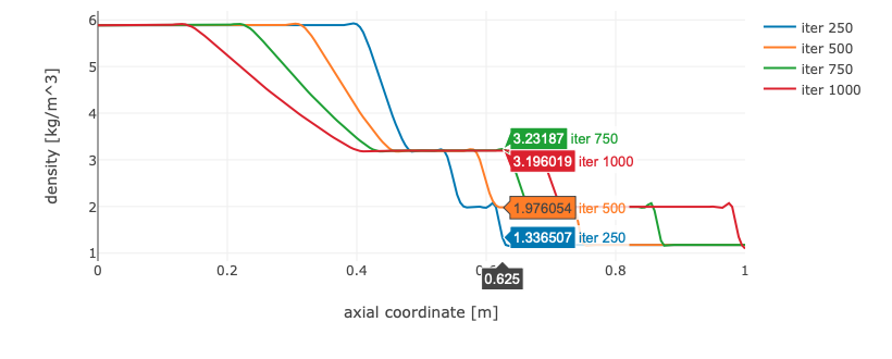
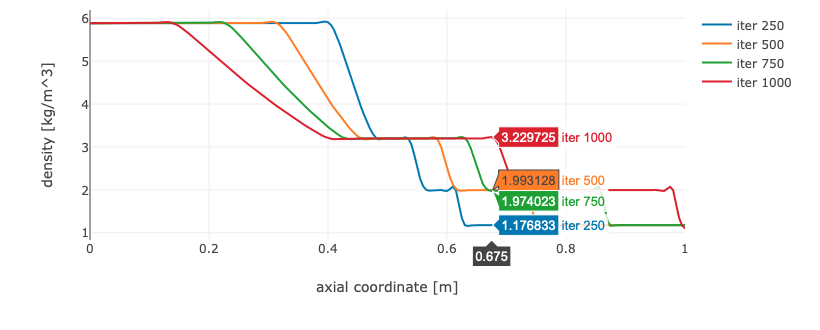
One way of finding the shock, head, and tail velocities is produce several solutions with a few time steps (e.g. 250) between each solution (run the solver multiple times). By default, all solutions are saved and can be plotted in the same graphs for comparison purposes using the flow data archive functionality in CFLOW post (see example below). The speed can be estimated from the distance traveled from the center of the tube.
Remember to export the solver state to a JSON-file when you are done with the task.
| Geometry definition |
| pipe type |
constant-area pipe, two regions (shock tube) |
| left-end coordinate |
0.0 |
| right-end coordinate |
1.0 m |
| interface coordinate |
0.5 m |
| pipe cross-section area |
not important - use d = 0.1 m |
| Mesh properties |
| Number of cells |
200 (refine later if needed) |
| Cell spacing |
uniform mesh |
| Numerics |
| Artificial damping (shocks) |
0.5 |
| Artificial damping (temperature) |
2.0 |
| Time-stepping mode |
time accurate (dt) |
| Time step |
1.e-6 s |
| Run parameters |
| Number of time steps |
Set the number of time steps to 250 (each time you press play, the solution will move forward in time 250 x 1.e-6 s) |
| Gas properties |
|
use the default settings for air |
| Initial flow field |
| Region 1 |
specify constant values in the driver section before the shock tube is started |
| Region 2 |
specify constant values in the driven section before the shock tube is started |
| Boundary conditions |
| Left-end boundary |
solid wall |
| Right-end boundary |
solid wall |
Assignment Report
In order to complete the assignment, a report should be written and handed in for assessment. A suggested report structure is given below.
For each of the tasks, report the following:
- Analytical solution
- you may include photos/scans of hand-written calculations if you want
- CFLOW solver settings
- you only need to report solver settings if you have used something else than the recommended settings for the task
- Solver convergence
- residual plot (found under convergence in the cflow solver)
- Do you consider the solution to be converged enough? Justify your answer
- Where there any problems getting the solver to converge for this specific case. If so, speculate on the cause for this behavior.
- Results
- Flow field plots (for example Mach number, temperature, pressure and/or any of the other available flow field variables if you find something that is particularly interesting) - flow field plots are found under postprocessing in the cflow solver
- Comment on what you see (are there any specific flow features that can be observed in the results)
- Discussion
- Are there any significant deviations from the analytical solution? If so, what is the reason for the deviations? (it might be difficult to answer exactly but a speculation will do)
- Are there any indications of numerical errors in the solution?
- wiggles in flow field data
- changes in total temperature for cases that should be adiabatic
- changes in total pressure for cases that should be isentropic
- other indications of numerical errors
When done, submit the report along with the exported JSON-files in Canvas