Case 08

Supersonic flow over a cylinder

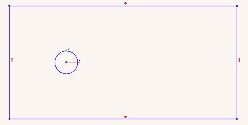
This problem includes inviscid compressible flow in two space dimensions. The geometric dimensions of the computational domain is given in the figure below and the problem consists of computing the 2D unsteady flow around the cylinder according to specifications below. The flow will include features such as compression regions, shocks, and expansion regions. A supersonic flow is imposed at the inlet boundary.

Figure 1: Overall view of computational domain, showing shape and extent of outer boundary

Literature review

Specifications

Supersonic flow over a cylinder is a classic problem for evaluation of the accuracy of numerical schemes and validation of numerical codes. The step is defined geometrically according to the figure above where the length \(L\) is set to 1.0. The flow is initialized with a pressure \(p=1.0\), density \(\rho=1.4\), and a Mach number of \(M=3.0\). The sudden start at Mach 3.0 will lead to the formation of a complex shock system and the problem is highly unstable. Therefore, an unsteady solver should be used.

The initial conditions are as follows:

initial flow
\(\rho\)	1.4 \(kg/m^3\)
\(p\)	1 \(Pa\)
\(u\)	3.0 \(m/s\)

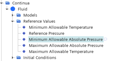
Note that since the initial pressure (and the pressure at the inlet and outlet) is set to 1.0, the temperature will be close to 0 Kelvin. The simulation will crash unless you set the lower limit of temperature and pressure to zero. Continua -> Physics 1 -> Reference Values -> Minimum Allowable Temperature / Minimum Allowable Absolute Pressure

Task 1

Do an inviscid simulation for the cylinder as specified above. Use stagnation inlet and pressure outlet boundary conditions.

Task 2

Investigate the effect of viscosity for the cylinder flow by running a viscous simulation using the Spallart-Almaras turbulence model.

Expected results and presentation

The flow field will contain compression regions, oblique shocks, and expansion fans. Although contour plots should be used for the visualization of these flow features it might be difficult to do a qualitative comparison of different simulations (simulations made using different meshes and numerical settings) and analytical results. Therefore, when comparing shock strength and location of flow features, it is recommended to extract data along axial lines at different \(y\) coordinates and compare the data in terms of \(xy\)-plots.

Grid generation guidelines

There should not be any large jump in cell sizes anywhere. The changes in cell size must be smooth otherwise you might run into problems with convergence.

The geometry can be generated in using the Create Rectangle and Create Circle tools

CFD guidelines

Some general guidelines for the simulation:

Don't forget to set the reference pressure to zero:

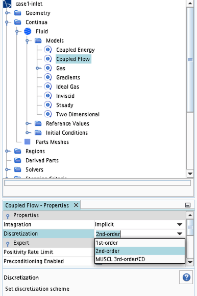
Continua -> Fluid -> Reference Values -> Reference Pressure

In your project, you should investigate the performance of different numerical schemes. The numerical scheme is modified under Continua -> Fluid -> Models -> Coupled Flow. Note, in case you have not renamed the physics entry under Continua, the default name is Physics 1.

Some of the cases, or at least some of the operation conditions for some cases, will have convergence problems due to flow instabilities. In case you get that type of solver behavior, try to find another convergence criterion by for example measuring forces or massflow. You may also consider updating the mesh as it is crucial to resolve important flow features to reach convergence.

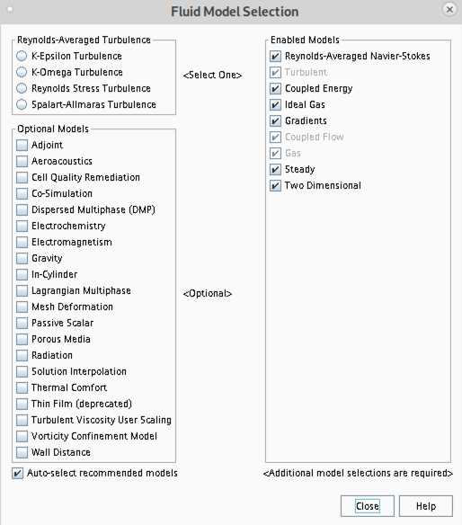
Some of the cases should be simulated using a viscous solver. Choose Turbulent instead of Inviscid when you select models and then select an appropriate turbulence model.

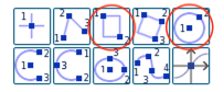
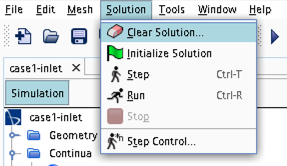
In case you would like to start your simulation from scratch, the flow field can be reset as indicated in the picture below (don't forget to initialize the flow field after the reset).

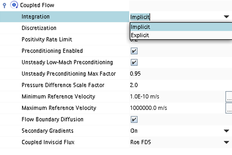
Time stepping approach (implicit/explicit) is selected under Continua -> Fluid -> Models -> Coupled Flow

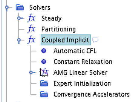
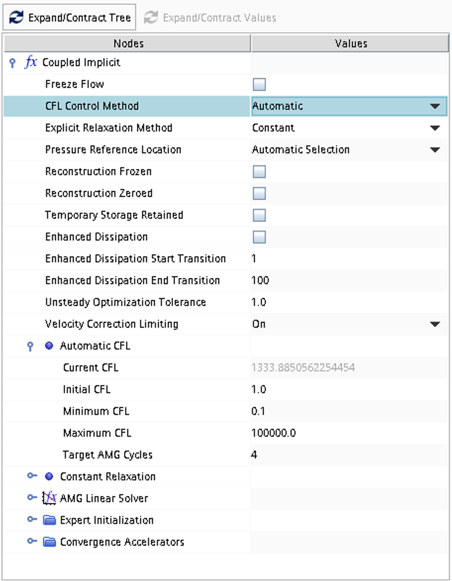
CFL number and other solver settings are found under Solver -> Coupled Implicit (or Solver -> Coupled Explicit)