Case 1

Inviscid Flow Through Engine Intake (steady state)

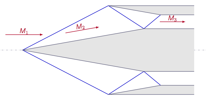
The task is to solve the flow field inside a supersonic engine intake (see Figure 1) both numerically using STAR-CCM+ and analytically. The flow can be assumed to be stationary, inviscid, compressible and two-dimensional.

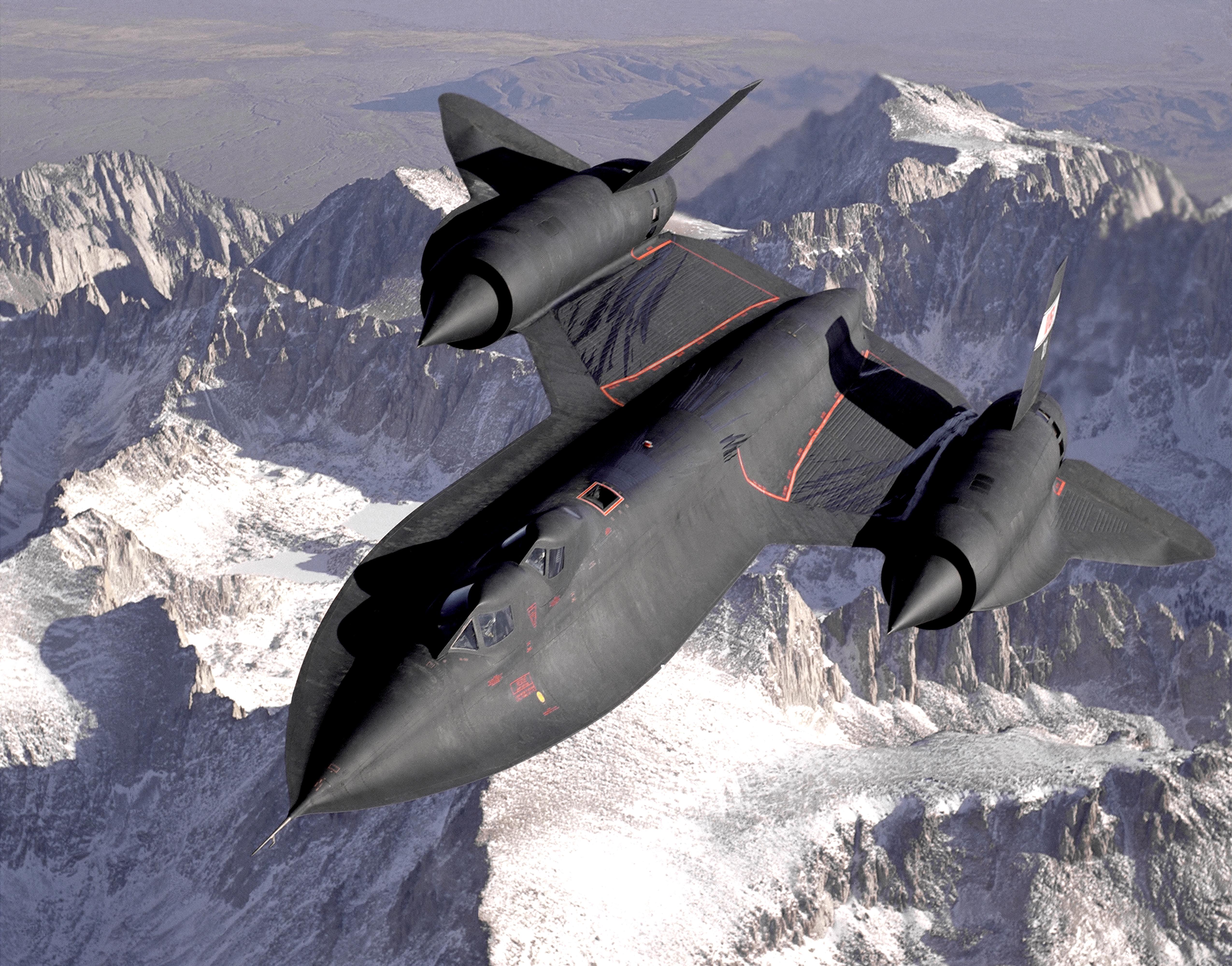
Lockheed SR-71 Blackbird — Figure 1: SR-71 (blackbird)
https://en.wikipedia.org/wiki/Lockheed_SR-71_Blackbird

schematic representation of engine intake — Figure 2: Schematic representation of engine intake

Literature review

Geometry specifications

The coordinates are given in Figure 3.

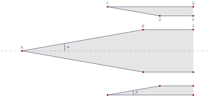
schematic representation of engine intake - coordinates — Figure 3: Intake coordinates (\(\alpha=\beta=10^\circ\))


Node  X (m)   Y (m)
A     0.0     0.0
B     7.0713  1.2469
C    10.0     1.2469
D     8.045   2.055
E    10.0     2.055
F     5.0     2.5918
G    10.0     2.5918

Since the geometry is symmetric, only one side of the intake needs to be resolved. In order to be able to apply the theory covered in the course directly to this geometry, it is set to be symmetric in the 2D plane (2D planar) rather than axi-symmetric which would be closer to reality. Note that for Task 2a, the computational domain needs to be stretched to the far field.

Specifications

For all tasks, ideal gas is assumed with \(\gamma\)=1.4, \(Pr\)=0.7, and \(\mu\)=0.

Task 1 (design point)
Calculate the inlet Mach number such that the first oblique shock exactly touches the outer edge (as seen in Figure 1). This can be done either analytically or numerically by changing the inlet boundary condition until the condition is met.
Inflow	\(M_{inlet}=?\), velocity in the axial direction
Ambient conditions	\(T_\infty=288\) K and \(p_\infty=1.0\) bar
Task 2
Inflow	\(M_{inlet}=30\)% higher than Task 1, velocity in the axial direction
Ambient conditions	\(T_\infty=288\) K and \(p_\infty=1.0\) bar
Task 3
Inflow	\(M_{inlet}=2\)% lower than Task 1, velocity in the axial direction
Ambient conditions	\(T_\infty=288\) K and \(p_\infty=1.0\) bar

Expected results

The solutions obtained should be presented in the form of pressure/Mach/entropy contour plots, showing any special features in the flow such as shocks, expansion fans etc. Based on the contour plots, explain what happens in the flow and why. Also, a comparison between the three cases should be made. Explain what the main differences are between the three studied cases. Which of the three cases have the lowest losses and why? Why do you think the intake is designed as it is? The explanations should be backed up with analytical calculations if possible.

Grid generation guidelines

There should not be any large jump in cell sizes anywhere. The changes in cell size must be smooth otherwise you might run into problems with convergence.

CFD guidelines

It is recommended that the flow field is initialized with the inlet conditions of Task 1. Besides checking the residuals, define an overall convergence measure that you think is reasonable.

Some general guidelines for the simulation:

Don't forget to set the reference pressure to zero:

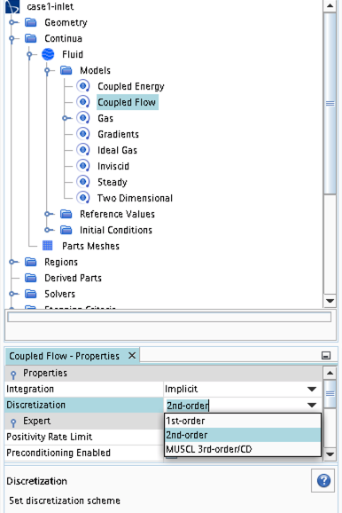
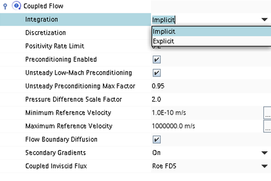
Continua -> Fluid -> Reference Values -> Reference Pressure

In your project, you should investigate the performance of different numerical schemes. The numerical scheme is modified under Continua -> Fluid -> Models -> Coupled Flow. Note, in case you have not renamed the physics entry under Continua, the default name is Physics 1.

Some of the cases, or at least some of the operation conditions for some cases, will have convergence problems due to flow instabilities. In case you get that type of solver behavior, try to find another convergence criterion by for example measuring forces or massflow. You may also consider updating the mesh as it is crucial to resolve important flow features to reach convergence.

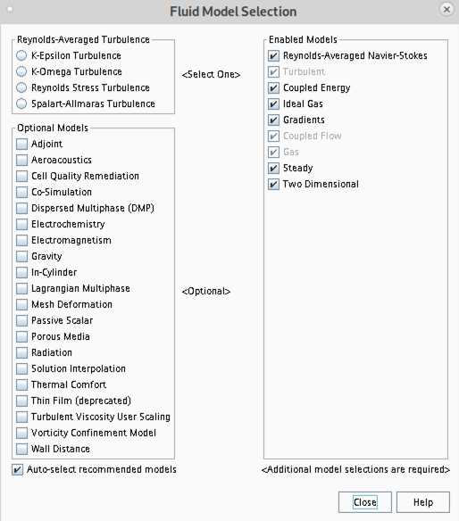
Some of the cases should be simulated using a viscous solver. Choose Turbulent instead of Inviscid when you select models and then select an appropriate turbulence model.

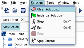
In case you would like to start your simulation from scratch, the flow field can be reset as indicated in the picture below (don't forget to initialize the flow field after the reset).

Time stepping approach (implicit/explicit) is selected under Continua -> Fluid -> Models -> Coupled Flow

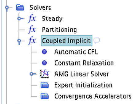
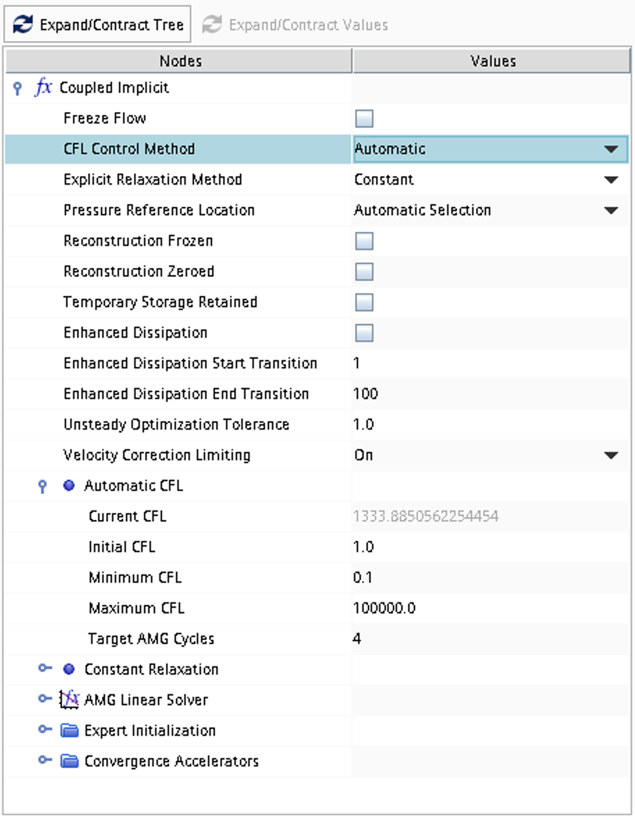
CFL number and other solver settings are found under Solver -> Coupled Implicit (or Solver -> Coupled Explicit)