Case 5
Supersonic flow over a biconvex airfoil
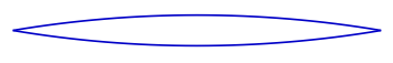
 The supersonic flow over a biconvex airfoil is investigated using STAR-CCM+. The solution obtained in STAR-CCM+ is compared with experimental data and an analytical solution. The pressure coefficient along the upper and lower surface of the airfoil is compared with measurements. Additionally, the shock pattern predicted in STAR-CCM+ is compared to a Schlieren image of the flow. The experimental data was obtained in a supersonic wind tunnel at KTH Royal Institute of Technology in Stockholm, Sweden. The biconvex airfoil geometry is shown in Figure 1.
Literature review
Suggested search topics
- Schlieren photography
- Supersonic flow around an airfoil
Computational domain
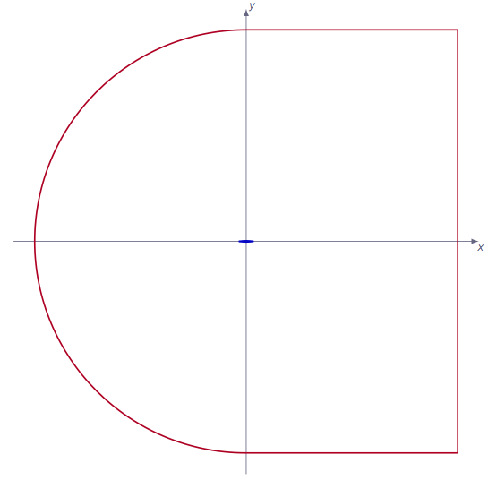
The extent of the domain is shown in Figure 2, As can be seen from the figure, the extent of the computational domain (red lines) is significantly larger than that of the airfoil (blue lines in the center of the figure). Typically, the computational domain ranges from -1m to 1m both in the \(x\) and \(y\) directions.
Airfoil Geometry
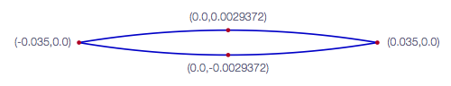
The coordinates needed to define the airfoil geometry are shown in Figure 3. In STAR-CCM+, define four coordinates according to the figure below, then use the Create Three-Point Circular Arc tool for the definition of the upper and lower airfoil surface.
Specifications
Case 5 consists of two tasks. The parameters for Task 1 and Task 2 are listed in Table 1 and Table 2, respectively.
Table 1: Parameters for Task 1
| Parameter | Value |
| Free stream Mach number | 2.3 [-] |
| Airfoil angle of attack | 1 [deg] |
| Free stream static pressure | 20 340 [Pa] |
| \(T_o\) | 295 [K] |
Table 2: Parameters for Task 2
| Parameter | Value |
| Free stream Mach number | 2.0 [-] |
| Airfoil angle of attack | 0 [deg] |
| Free stream static pressure | 32 506 [Pa] |
| \(T_o\) | 295 [K] |
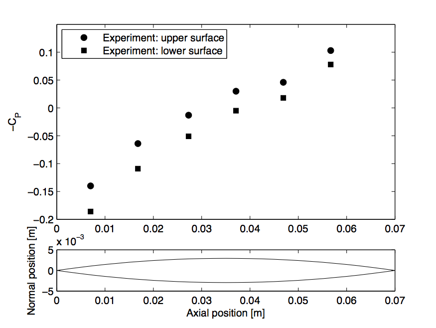
For both tasks, ideal gas is assumed. The axial positions where the static pressure was measured in the experiment are shown in Fig. 4. For Task 1, the pressure coefficient along the upper and lower surface of the airfoil should be compared to the experimental results presented in Table 3.
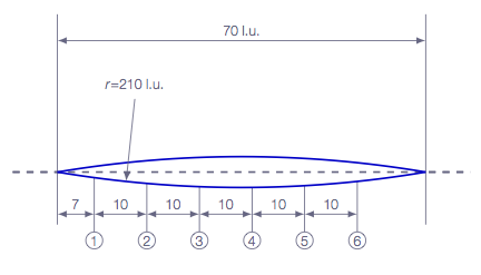
Table 3: Experimental measurements of the pressure coefficient along the upper and lower surface in Task 1
| Position \(x/c\) |
Pressure coefficient upper surface |
Pressure coefficient lower surface |
| 0.10 | 0.140 | 0.186 |
| 0.24 | 0.064 | 0.109 |
| 0.39 | 0.013 | 0.051 |
| 0.53 | -0.030 | 0.005 |
| 0.67 | -0.046 | -0.018 |
| 0.81 | -0.103 | -0.078 |
The pressure coefficient is calculated as shown in Equation 1
$$C_P = \frac{p-p_\infty}{q_\infty} = \frac{p-p_\infty}{\frac{1}{2}\rho_\infty V_\infty^2}$$where \(p\), \(q\), \(\rho\), \(V\) are the static pressure, dynamic pressure, density and velocity, respectively. The subscript \(\infty\) denotes a value measured far upstream where the flow is not disturbed by the airfoil. The experimental data is plotted in Figure 5. Note that \(-C_p\) is used on the y-axis.
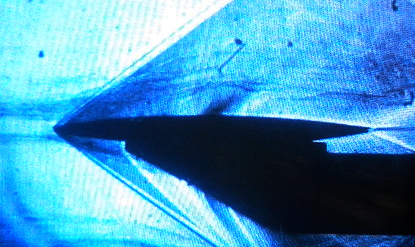
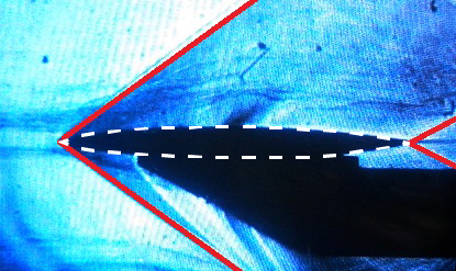
A schlieren image of the flow around the biconvex airfoil in Task 2 is shown in Figure 6. A schlieren image visualizes regions with high density gradients. Figures 6a and 6b show the same image but in Figure 6b the outline of the airfoil is indicated (dotted white line) and the shocks are highlighted (solid red lines). The outline of the shocks should be compared with the shock pattern obtained in STAR-CCM+. It should be noted that in the experiments there are additional shocks from the stand which keeps the airfoil in place, and reflections are shown from the wind tunnel walls. These additional shocks can be ignored when comparing the results.
Expected results and presentation
- For Task 1 and Task 2, the flow field should be presented in the form of density, pressure and Mach contour plots (zoomed in on regions where interesting flow features occur).
- A comparison should be made of the experimental values of the pressure coefficient, an analytical solution and the solution obtained in STAR-CCM+. Guidelines on how to calculate the analytical solution of the pressure coefficient along the surface of the biconvex airfoil are given in a separate section below.
Note: An equation based on linearized supersonic theory is shown in the reference. This can be presented in your report under the condition that you show how it is derived. However, it should not be presented instead of the approach described below, but it can be shown as an additional comparison. - The shock position in Task 2 should be compared to the best of your ability with Figure 6a.
- Additional comparisons you can think of ...
Analytical calculation of the pressure coefficient
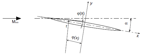
To calculate the analytical pressure coefficient along the upper and lower surface of the airfoil, the Mach number and pressure behind the first oblique shocks needs to be calculated. Behind the oblique shocks, the flow is turned gradually by Prandtl-Meyer expansion. The angle \(\psi(x)\) is the angle between a line tangential to the surface and the chord line and needs to be calculated using the information provided in Figure 4 and Figure 7.
It should be noted that neither the experimental measurements or the analytical solution are exact. For example, in the experiment, the airfoil used to obtain the experimental values of the pressure coefficient had a slightly rounded leading edge. The analytical solution and the solution obtained using STAR-CCM+ neglects any influence of the boundary layer. Additional sources of error are present. However, it is sufficient to know that the values from none of the methods are exact.
Grid generation guidelines
There should not be any large jump in cell sizes anywhere. The changes in cell size must be smooth otherwise you might run into problems with convergence.
CFD guidelines
Some general guidelines for the simulation:
- Don't forget to set the reference pressure to zero:
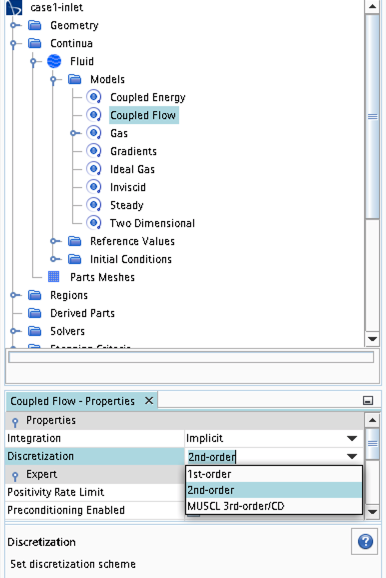
Continua -> Fluid -> Reference Values -> Reference Pressure- In your project, you should investigate the performance of different numerical schemes. The numerical scheme is modified under
Continua -> Fluid -> Models -> Coupled Flow. Note, in case you have not renamed the physics entry underContinua, the default name isPhysics 1.
- Some of the cases, or at least some of the operation conditions for some cases, will have convergence problems due to flow instabilities. In case you get that type of solver behavior, try to find another convergence criterion by for example measuring forces or massflow. You may also consider updating the mesh as it is crucial to resolve important flow features to reach convergence.
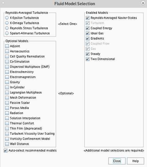
- Some of the cases should be simulated using a viscous solver. Choose
Turbulentinstead ofInviscidwhen you select models and then select an appropriate turbulence model.
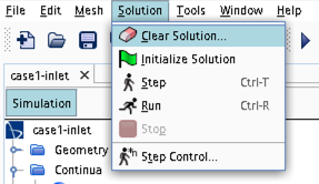
- In case you would like to start your simulation from scratch, the flow field can be reset as indicated in the picture below (don't forget to initialize the flow field after the reset).
- Time stepping approach (implicit/explicit) is selected under
Continua -> Fluid -> Models -> Coupled Flow
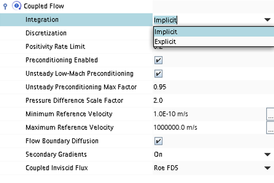
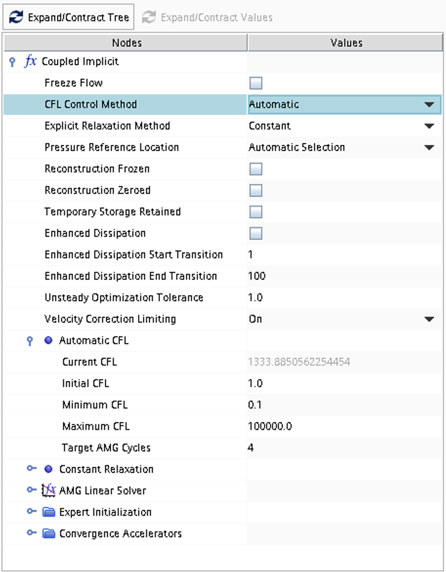
- CFL number and other solver settings are found under
Solver -> Coupled Implicit(orSolver -> Coupled Explicit)
References
- KTH Mechanics Laboration Instructions. Pressure distribution on a biconvex airfoil in supersonic flow.