Chapter 7
Unsteady Wave Motion
Unsteady Wave Motion
Overview
So far, we have only studied waves under steady state conditions, i.e. stationary normal shocks, expansion fans and Mach waves. In chapter 7 we will be introduced to unsteady waves. Chapter 7 starts with deriving relations for moving normal shocks then theory related to acoustic wave propagation is presented and finally something that is referred to as finite nonlinear waves is discussed. The shock tube is an application where all sorts of traveling waves are present. Due to the simplicity of the shock tube and the fact that the traveling waves may be treated as one-dimensional makes it a good application for analytical analysis and therefore the shock tube is used as an example throughout chapter 7. In the end of the chapter when all types of traveling waves present in the shock tube has been introduced, the shock tube relations are derived and discussed.
Online Flow Calculator

Sections of the online flow calculator for compressible flow problems CFLOW related to this chapter:
- Section 1: Gas Relations
- Section 2: Total Flow Properties
- Section 3: Normal Shock Relations
- Section 9: Unsteady Wave Motion
- Section 10: The Shock Tube
The CFLOW finite-volume quasi-1D solver can also be used to study the problems in this chapter.
Chapter Roadmap
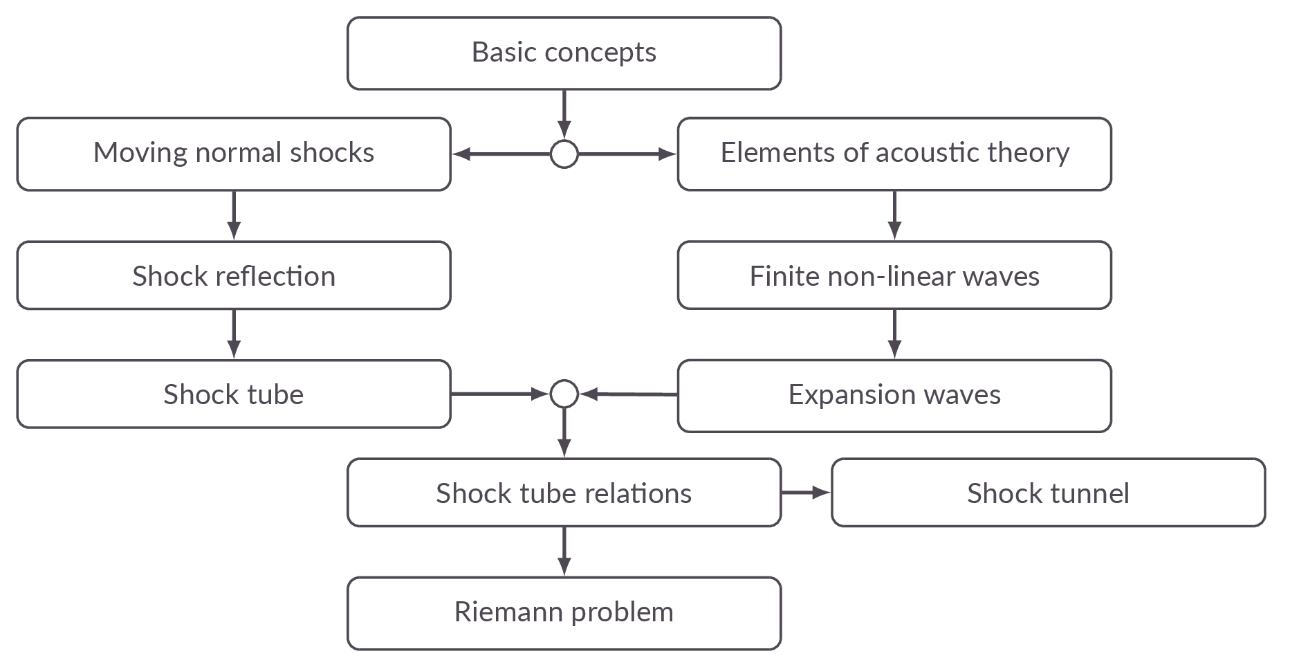
Sections
7.2 Moving Normal Shock Waves
The governing equations for a moving normal shock wave are presented. A normal shock moves with the velocity \(W\) in a stagnant fluid. In a frame of reference following the normal shock we will see a fluid motion ahead of the shock with velocity \(W\) relative to the shock and the velocity of the fluid behind the wave (relative to the wave) will be \((W-u_p)\), where \(u_p\) is the induced velocity. With this in mind, the governing equations are easily obtained from the normal shock equations presented in Chapter 3.
$$\rho_1 W = \rho_2(W-u_p)$$ $$p_1+\rho_1 W^2 = p_2 +\rho_2(W-u_p)^2$$ $$h_1+\frac{W^2}{2} = h_2 + \frac{(W+u_p)^2}{2} $$It is shown that the Hugoniot equation can be derived directly from these relations which implies that the thermodynamic relations are the same in the new frame of reference.
Expressions for calculation of the temperature and density ratios over the shock wave are derived. The expressions are based on the pressure ratio over the shock wave (the corresponding relations for stationary normal shocks presented in Chapter 3 where all based on the freestream Mach number ahead of the shock).
An expression for the calculation of the induced flow velocity \(u_p\) is derived. Again the relation is based on the pressure ratio over the moving shock. It turns out that if the shock becomes infinitely strong \(p_2/p_1\rightarrow\infty\), the induced Mach number approaches a finite value
$$\lim_{\frac{p_2}{p_1}\rightarrow \infty} M_p\rightarrow \sqrt{\frac{2}{\gamma(\gamma-1)}}$$For air with \(\gamma=1.4\), the limiting value is 1.89. The fact that there is a limit to how high Mach number that can be induced by the moving shock wave is interesting as such but the example above also shows that the limiting value is a high supersonic value.
7.3 Reflected Shock Wave
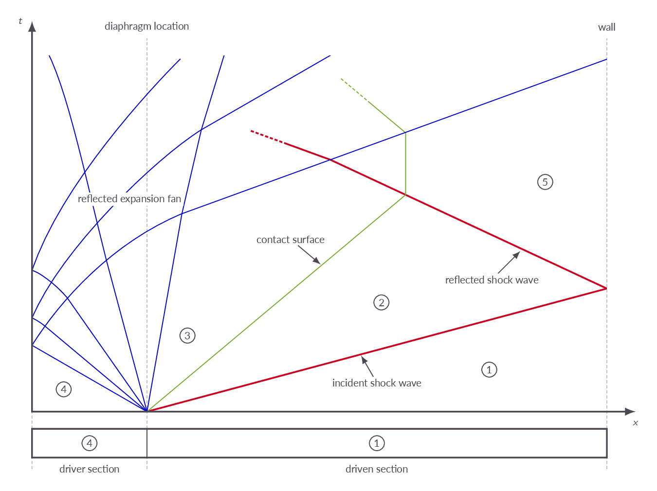
Shock wave reflection is exemplified by events in the shock tube application. When the incident shock wave, generated when the diaphragm in the shock tube separating the two flow states bursts, approaches the right wall of the shock tube, the fluid behind the shock wave has a velocity relative to the wall equal to the induced flow velocity \(u_p\). Of course the flow can not go through the wall and therefore a shock propagating in the opposite direction is generated at the instant when the incident shock reaches the wall. The reflected shock is set up such that it brings the fluid behind it to rest and thus the fluid near the wall is standing still.
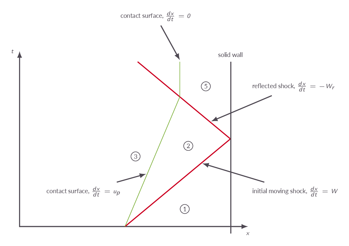
The governing equations for the reflected shock are presented
$$\rho_2 (W_r+u_p)=\rho_5 W_r$$ $$p_2+\rho_2(W_r+u_p)^2=p_5+\rho_5 W_r^2$$ $$h_2+\frac{1}{2}(W_r+u_p)^2=h_5+\frac{1}{2}W_r^2$$A relation between the Mach number of the reflected shock and the Mach number of the incident shock is presented at the end of the section. The derivation is left for the reader to do. Since the derivation is a bit tricky it is provided in pdf format in the document archive at the bottom of this page.
$$\frac{M_r}{M_r^2-1}=\frac{M_s}{M_s^2-1}\sqrt{1+\frac{2(\gamma-1)}{(\gamma+1)^2}(M_s^2-1)\left(\gamma+\frac{1}{M_s^2}\right)}$$7.4 Physical Picture of Wave Propagation
Wave propagation in one dimension is discussed as an introduction to the sections to follow. The concept finite wave is introduced.
7.5 Elements of Acoustic Theory
Propagation of acoustic waves are described as a natural part of the wave propagation section. An approximate equation governing the propagation of acoustic waves is derived using linearization. The starting point is the governing equations on differential form derived in Chapter 6. It is shown that in order to fulfill the wave equation, the waves must propagate with a constant velocity namely the speed of sound in the fluid in which the wave propagates.
Acoustic waves summarized:
- \(\Delta \rho\), \(\Delta u\), etc - very small
- All parts of the wave propagate with the same velocity \(a_\infty\)
- The wave shape stays the same
- The flow is governed by linear relations
7.6 Finite (Nonlinear) Waves
The discussion of wave propagation is continued with cases where the perturbations are not necessarily small, as was the case for the acoustic waves. Such waves, with significant or even large perturbations is what the author refer to as finite waves. For these finite waves nonlinearities may be significant and thus the linear relations obtained for the acoustic waves will not be adequate to use. Equations governing the propagation of finite waves are derived - again starting from the flow equations on differential form first presented in Chapter 6.
Analyzing the equations, it is observed that for waves moving along specific paths, the partial differential equations can be reduced to ordinary differential equations. These paths are referred to as characteristic lines and the technique introduced is the basis for the method of characteristics, which is of great importance for compressible flow analysis. From the characteristic lines, the Riemann invariants are obtained and it is showed how the Riemann invariants can be used for a calorically perfect gas to calculate the flow velocity and speed of sound in a location.
Finite nonlinear waves summarized:
- \(\Delta \rho\), \(\Delta u\), etc - can be large
- Each local part of the wave propagates at the local velocity (\(u+a\))
- The wave shape changes with time
- The flow is governed by non-linear relations
7.7 Incident and Reflected Expansion Waves
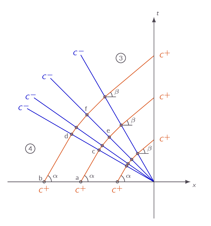
Again, the shock tube is used for illustration of traveling waves. In this section we sill learn how to analyze the expansion wave going to the left in the shock tube. The framework set up in the previous section based on characteristics and Riemann invariants is used to derive expressions relating the flow state into which the expansion wave is propagating (4) to the region behind the expansion region (3). Since both region 3 and 4 are regions with constant flow properties it can be shown that
constant flow properties in region 4:
$$J^+_a=J^+_b$$\(J^+\) invariants constant along \(C^+\) characteristics:
$$J^+_a=J^+_c=J^+_e$$ $$J^+_b=J^+_d=J^+_f$$since \(J^+_a=J^+_b\) this also implies \(J^+_e=J^+_f\)
\(J^-\) invariants constant along \(C^-\) characteristics:
$$J^-_c=J^-_d$$ $$J^-_e=J^-_f$$$$u_e=\frac{1}{2}(J^+_e+J^-_e),\ u_f=\frac{1}{2}(J^+_f+J^-_f),\ \Rightarrow u_e=u_f$$
$$a_e=\frac{\gamma-1}{4}(J^+_e-J^-_e),\ a_f=\frac{\gamma-1}{4}(J^+_f-J^-_f),\ \Rightarrow\ a_e=a_f$$
- The start and end conditions are the same for all \(C^+\) lines
- \(J^+\) invariants have the same value for all \(C^+\) characteristics
- \(C^-\) characteristics are straight lines in \(xt\)-space
- Simple expansion waves centered at \((x,t)=(0,0)\)
7.8 Shock Tube Relations
The shock tube problem is now completely defined since we can analyze all waves in the system. Combining the moving shock wave equations with the expansion region relations derived in the previous section it is now possible to derive an expression for the pressure ratio \(p_4/p_1\), i.e. the initial states in the shock tube.
$$\frac{p_4}{p_1}=\frac{p_2}{p_1}\left\{ 1 -\frac{(\gamma_4-1)(a_1/a_4)(p_2/p_1-1)}{\sqrt{2\gamma_1\left[2\gamma_1+(\gamma_1+1)(p_2/p_1-1)\right]}}\right\}^{-2\gamma_4/(\gamma_4-1)}$$- \(p_2/p_1\) as implicit function of \(p_4/p_1\)
- for a given \(p_4/p_1\), \(p_2/p_1\) will increase with decreased \(a_1/a_4\)
7.9 Finite Compression Waves
With finite expansion waves covered in the previous section, finite compression waves are now discussed. In contrast to the expansion region that always spread in space over time the individual waves in the compression region will approach each other over time and the compression region will coalesce into a shock wave.
Study Guide
The questions below are intended as a "study guide" and may be helpful when reading the text book.
Moving Normal Shocks
- What is the connection between a stationary and a moving normal shock?
- Think about the oblique shock from an object flying through the air at supersonic velocity. How will an observer on the ground experience the shock wave?
- Suppose you are given a problem in which there is a moving normal shock but the gas velocities are non-zero on both sides of the shock. How would you transform the problem so as to make it simpler to solve?
- Is the Hugoniot equation valid for a moving normal shock?
- For normal shock moving into a stagnant calorically perfect gas, how can we apply the formulas for a stationary normal shock?
- Derive an the following expression for the induced flow velocity behind a moving shock $$u_p=\dfrac{a_1}{\gamma}\left(\dfrac{p_2}{p_1}-1\right)\left[\dfrac{\dfrac{2\gamma}{\gamma+1}}{\dfrac{p_2}{p_1}+\dfrac{\gamma-1}{\gamma+1}}\right]^{1/2}$$
- Describe what happens when a moving normal shock hits a solid wall.
- A stationary normal shock with upstream Mach number \(M_1\) (\(M_1>1\)) is compared to a moving normal shock, traveling with Mach number \(M_s\) into quiescent (non-moving) air. If \(M_1=M_s\), is there any physical difference between the two shock waves apart from the fact that they have different speeds relative to the observer?
- The moving shock is an adiabatic process in the same way as a stationary normal shock is adiabatic. Does this mean that total enthalpy is constant over the moving shock? Explain why/why not.
- Can a moving normal shock travel at a speed lower than the speed of sound? Explain why/why not.
- What is the maximum Mach number of the induced flow behind a moving shock?
- In Formulas, Tables & Graphs, check formulas on pages (19-20). You should recognize the relation between the shock Mach number \(M_s\) and the shock pressure ratio \(p_2/p_1\), the formula for the induced velocity up and the formulas for the temperature and density ratios. Also the formula for the Mach number \(M_R\) of a reflected shock and how its velocity \(W_R\) is computed.
Finite Non-Linear Waves
- Which two equations are used to derive the Riemann Invariants?
- What are the assumptions in this case?
- How are the two characteristic curves \(C^+\) and \(C^-\) defined?
- Describe the Method of Characteristics (MOC) as a means of computing the time evolution of inviscid flow.
- Can we apply MOC when there are shocks present?
- Describe a left-going simple expansion wave in terms of the characteristics \(C^+\), \(C^-\) and Riemann invariants \(J_+\), \(J_-\).
- Derive the expansion wave relations
- An unsteady expansion wave is traveling inside a tube in which viscous effects are found to be negligible. Which of the following variables are constant throughout the expansion wave?
- pressure
- temperature
- entropy
- density
- In Formulas, Tables & Graphs, check formulas on pages (21-22). You should recognize the relations governing a left-going simple expansion wave where condition 4 is the original stagnant condition on the left side (the head of the expansion wave) and condition 3 is the tail of the expansion wave.
The Shock Tube
- Which types of waves or discontinuities are generated in shock tubes?
- Which is the driver section and which is the driven section?
- How does the shock tube solution depend on \(x\) and \(t\)?
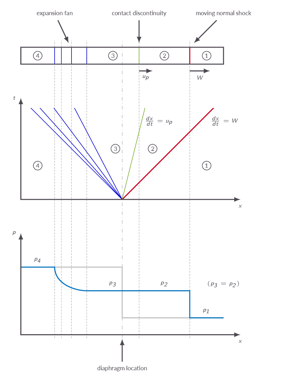
- Draw a typical solution in an \(x\)-\(t\) diagram, where you describe the phenomena and how they are placed in relation to each other and in relation to the driver section and driven section.
- In shock tubes, unsteady contact discontinuities are sometimes found. Describe in words what they are and under which circumstances they may be formed. Which of the variables \(p\), \(T\), \(\rho\), \(u\), \(s\) is/are necessarily continuous across such a contact discontinuity?
- Is the expansion fan an isentropic or non-isentropic wave?
- What is the shock tube used for in laboratories around the world?
- What types of waves or discontinuities are generated in a shock tube with two initially stagnant regions at different pressure (separated by a thin membrane which is removed very quickly)?
- In Formulas, Tables & Graphs, check formulas on page (22). You should recognize the shock tube solution for calorically perfect gas. Note that since conditions 1 and 4 usually are given, the equation must be solved iteratively to obtain the intermediate pressure \(p_2\ (=p_3)\). Once this is known, the expansion fan, the contact discontinuity and the moving shock are all defined.
Acoustic Theory
- Which flow equations and what assumptions are used to derive the acoustic equations?
- How can the acoustic equations be combined into one single (classical) wave equation?
- Give the general solution to the classical wave equation in one space dimension and time.
- Describe how the relations between pressure, density and velocity amplitudes may be obtained.
- What is the difference between acoustic waves and other types of waves such as shock waves and expansion waves?